by Annette Gerritsen, Ph.D.
Cross-tabulation in cohort studies
Assume you have just done a cohort study. How do you actually do the cross-tabulation to calculate the cumulative incidence in both groups?
Best is to always put the outcome variable (disease yes/no) in the columns and the exposure variable in the rows. In other words, put the dependent variable–the one that describes the problem under study–in the columns. And put the independent variable–the factor assumed to cause the problem–in the rows.
Let’s take as example a cohort study used to see whether there is a causal relationship between the use of a certain water source and the incidence of diarrhea among children under five in a village with different water sources. In this case, the variable diarrhea (yes/no) should be in the columns. The variable water source (suspected/other) should be in the rows.
SPSS will put the lowest value of the variable in the first column or row. So in order to get those with diarrhea in the first column you should label ‘diarrhea’ as 1 and ‘no diarrhea’ as 2. The same is true for the exposure variable: label the ‘suspected water source’ as 1 and the ‘other water source’ as 2.
You will then be able to calculate the cumulative incidence (risk of developing the disease) among those with the exposure: a / (a + b) and among those without the exposure: c / (c + d).
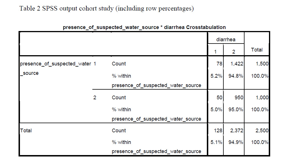
In the case of the diarrhea study (Table 1), you could calculate the cumulative incidence of diarrhea among those exposed to the suspected water source, which would be (78 / 1,500 =) 5.2%.
You can also do this for those exposed to other water sources, which would be (50 / 1,000 =) 5.0%.

SPSS can give you these percentages immediately (in cell ‘a’ and ‘c’ respectively), when you ask to display row percentages in the Cells option (Table 2).

Cross-tabulation in Case-Control Studies
When you have used a case-control design for the diarrhea study, the actual cross-tabulation is quite similar, only “presence of diarrhea yes/no”, is now changed into “cases” and “controls.
Label the cases as 1, and the controls as 2. Be aware that row percentages have no meaning in terms of occurrence of disease in case-control studies. This is because in case-control studies the researcher determines how many patients and how many controls are included.
The ratio between the number of patients and controls (e.g. 2 : 1 or 4 : 1) influences the row percentages. So in a case-control study, the cumulative incidence cannot be calculated.
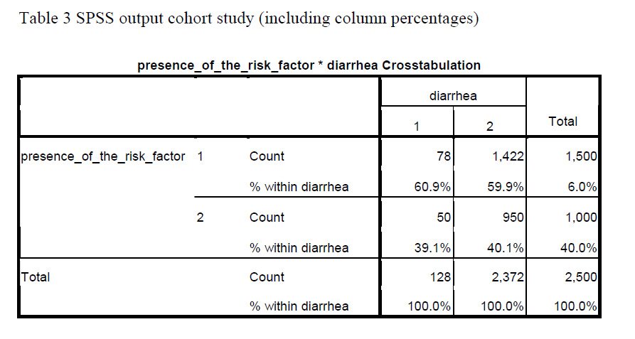
When having conducted a case-control study, you can ask to display column percentages. That gives you the proportion of those exposed to the suspected water source among the cases (in cell ‘a’) and among the controls (in cell ‘b’).
Table 3 gives the SPSS output for the same diarrhea study assuming that it had a case-control design. Using the data provided, (78 / 128 =) 60.9% of the cases were exposed to the suspected water source, while this was (1,422 / 2,372 =) 59.9% of the controls (asked for column percentages).

Another article will be devoted to measures of association: How do you actually compare cumulative incidence rates in cohort studies? And what measure of association can be used in case-control studies?
About the Author: With expertise in epidemiology, biostatistics and quantitative research projects, Annette Gerritsen, Ph.D. provides services to her clients focussing on the methodological soundness of each phase of an epidemiological study to ensure getting valid answers to the proposed research questions. She is the founder of Epi Result.
I recently received this question:
I have scale which I want to run Chronbach’s alpha on. One response category for all items is ‘not applicable’. I want to run Chronbach’s alpha requiring that at least 50% of the items must be answered for the scale to be defined. Where this is the case then I want all missing values on that scale replaced by the average of the non-missing items on that scale. Is this reasonable? How would I do this in SPSS?
My Answer:
In RELIABILITY, the SPSS command for running a Cronbach’s alpha, the only options for Missing Data (more…)
 If you are a SPSS, SAS, or Stata user who finds yourself needing to use R (I mean, it’s free), I just found this great website: http://statmethods.net/index.html.
Regression models are just a subset of the General Linear Model, so you can use GLM procedures to run regressions. It is what I usually use.
But in SPSS there are options available in the GLM and Regression procedures that aren’t available in the other. How do you decide when to use GLM and when to use Regression?
GLM has these options that Regression doesn’t: (more…)
In addition to the five listed in this title, there are quite a few other options, so how do you choose which statistical software to use?
The default is to use whatever software they used in your statistics class–at least you know the basics.
And this might turn out pretty well, but chances are it will fail you at some point. Many times the stat package used in a class is chosen for its shallow learning curve, (more…)
SPSS Variable Labels and Value Labels are two of the great features of its ability to create a code book right in the data set. Using these every time is good data analysis practice.
SPSS doesn’t limit variable names to 8 characters like it used to, but you still can’t use spaces, and it will make coding easier if you keep the variable names short. You then use Variable Labels to give a nice, long description of each variable. On questionnaires, I often use the actual question.
There are good reasons for using Variable Labels right in the data set. I know you want to get right to your data analysis, but using Variable Labels will save so much time later.
1. If your paper code sheet ever gets lost, you still have the variable names.
2. Anyone else who uses your data–lab assistants, graduate students, statisticians–will immediately know what each variable means.
3. As entrenched as you are with your data right now, you will forget what those variable names refer to within months. When a committee member or reviewer wants you to redo an analysis, it will save tons of time to have those variable labels right there.
4. It’s just more efficient–you don’t have to look up what those variable names mean when you read your output.
Variable Labels
The really nice part is SPSS makes Variable Labels easy to use:
1. Mouse over the variable name in the Data View spreadsheet to see the Variable Label.
2. In dialog boxes, lists of variables can be shown with either Variable Names or Variable Labels. Just go to Edit–>Options. In the General tab, choose Display Labels.
3. On the output, SPSS allows you to print out Variable Names or Variable Labels or both. I usually like to have both. Just go to Edit–>Options. In the Output tab, choose ‘Names and Labels’ in the first and third boxes.
Value Labels
Value Labels are similar, but Value Labels are descriptions of the values a variable can take. Labeling values right in SPSS means you don’t have to remember if 1=Strongly Agree and 5=Strongly Disagree or vice-versa. And it makes data entry much more efficient–you can type in 1 and 0 for Male and Female much faster than you can type out those whole words, or even M and F. But by having Value Labels, your data and output still give you the meaningful values.
Once again, SPSS makes it easy for you.
1. If you’d rather see Male and Female in the data set than 0 and 1, go to View–>Value Labels.
2. Like Variable Labels, you can get Value Labels on output, along with the actual values. Just go to Edit–>Options. In the ‘Output Labels’ tab, choose ‘Values and Labels’ in the second and fourth boxes.


