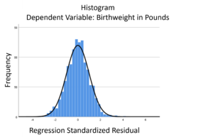
The linear model normality assumption, along with constant variance assumption, is quite robust to departures. That means that even if the  assumptions aren’t met perfectly, the resulting p-values and confidence intervals will still be reasonable estimates.
This is great because it gives you a bit of leeway to run linear models, which are intuitive and (relatively) straightforward. This is true for both linear regression and ANOVA.
You do need to check the assumptions anyway, though. You can’t just claim robustness and not check. Why? Because some departures are so far off that the p-values and confidence intervals become inaccurate. And in many cases there are remedial measures you can take to turn non-normal residuals into normal ones.
But sometimes you can’t.
Sometimes it’s because the dependent variable just isn’t appropriate for a linear model. The (more…)
When your dependent variable is not continuous, unbounded, and measured on  an interval or ratio scale, linear models don’t fit. The data just will not meet the assumptions of linear models. But there’s good news, other models exist for many types of dependent variables.
Today I’m going to go into more detail about 6 common types of dependent variables that are either discrete, bounded, or measured on a nominal or ordinal scale and the tests that work for them instead. Some are all of these.
(more…)
Predictor variables in statistical models can be treated as either continuous or categorical.
Usually, this is a very straightforward decision.
Categorical predictors, like treatment group, marital status, or highest educational degree should be specified as categorical.
Likewise, continuous predictors, like age, systolic blood pressure, or percentage of ground cover should be specified as continuous.
But there are numerical predictors that aren’t continuous. And these can sometimes make sense to treat as continuous and sometimes make sense as categorical.
(more…)
Most of us know that binary logistic regression is appropriate when the outcome variable has two possible outcomes: success and failure.
There are two more situations that are also appropriate for binary logistic regression, but they don’t always look like they should be.
(more…)
There are quite a few types of outcome variables that will never meet ordinary linear model’s assumption of normally distributed residuals. A non-normal outcome variable can have normally distribued residuals, but it does need to be continuous, unbounded, and measured on an interval or ratio scale. Categorical outcome variables clearly don’t fit this requirement, so it’s easy to see that an ordinary linear model is not appropriate. Neither do count variables. It’s less obvious, because they are measured on a ratio scale, so it’s easier to think of them as continuous, or close to it. But they’re neither continuous or unbounded, and this really affects assumptions.
Continuous variables measure how much. Count variables measure how many. Count variables can’t be negative—0 is the lowest possible value, and they’re often skewed–so severly that 0 is by far the most common value. And they’re discrete, not continuous. All those jokes about the average family having 1.3 children have a ring of truth in this context.
Count variables often follow a Poisson or one of its related distributions. The Poisson distribution assumes that each count is the result of the same Poisson process—a random process that says each counted event is independent and equally likely. If this count variable is used as the outcome of a regression model, we can use Poisson regression to estimate how predictors affect the number of times the event occurred.
But the Poisson model has very strict assumptions. One that is often violated is that the mean equals the variance. When the variance is too large because there are many 0s as well as a few very high values, the negative binomial model is an extension that can handle the extra variance.
But sometimes it’s just a matter of having too many zeros than a Poisson would predict. In this case, a better solution is often the Zero-Inflated Poisson (ZIP) model. (And when extra variation occurs too, its close relative is the Zero-Inflated Negative Binomial model).
ZIP models assume that some zeros occurred by a Poisson process, but others were not even eligible to have the event occur. So there are two processes at work—one that determines if the individual is even eligible for a non-zero response, and the other that determines the count of that response for eligible individuals.
The tricky part is either process can result in a 0 count. Since you can’t tell which 0s were eligible for a non-zero count, you can’t tell which zeros were results of which process. The ZIP model fits, simultaneously, two separate regression models. One is a logistic or probit model that models the probability of being eligible for a non-zero count. The other models the size of that count.
Both models use the same predictor variables, but estimate their coefficients separately. So the predictors can have vastly different effects on the two processes.
But a ZIP model requires it be theoretically plausible that some individuals are ineligible for a count. For example, consider a count of the number of disciplinary incidents in a day in a youth detention center. True, there may be some youth who would never instigate an incident, but the unit of observation in this case is the center. It is hard to imagine a situation in which a detention center would have no possibility of any incidents, even if they didn’t occur on some days.
Compare that to the number of alcoholic drinks consumed in a day, which could plausibly be fit with a ZIP model. Some participants do drink alcohol, but will have consumed 0 that day, by chance. But others just do not drink alcohol, so will never have a non-zero response. The ZIP model can determine which predictors affect the probability of being an alcohol consumer and which predictors affect how many drinks the consumers consume. They may not be the same predictors for the two models, or they could even have opposite effects on the two processes.
The assumptions of normality and constant variance in a linear model (both OLS regression and ANOVA) are quite robust to departures. That means that even if the assumptions aren’t met perfectly, the resulting p-values will still be reasonable estimates.
But you need to check the assumptions anyway, because some departures are so far off that the p-values become inaccurate. And in many cases there are remedial measures you can take to turn non-normal residuals into normal ones.
But sometimes you can’t.
Sometimes it’s because the dependent variable just isn’t appropriate for a linear model. The (more…)
 assumptions aren’t met perfectly, the resulting p-values and confidence intervals will still be reasonable estimates.
