Same Statistical Models, Different (and Confusing) Output Terms

Learning how to analyze data can be frustrating at times. Why do statistical software companies have to add to our confusion?

I do not have a good answer to that question. What I will do is show examples. In upcoming blog posts, I will explain what each output means and how they are used in a model.

We will focus on ANOVA and linear regression models using SPSS and Stata software. As you will see, the biggest differences are not across software, but across procedures in the same software.

The outcome variable is BMI (body mass index) and the predictor is a categorical variable for body frame: small, medium and large.

OneWay ANOVA Output

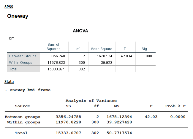
We could run this model through the Oneway ANOVA procedure.  This is the ANOVA table output.

Both tables have identical Sums of Squares, df, MS, F, and p-values. The one hypothesis test here is testing the null hypothesis that the three frame groups have the same mean BMI. This test is labeled “Between Groups” in this output.

ANOVA/General Linear Model Output

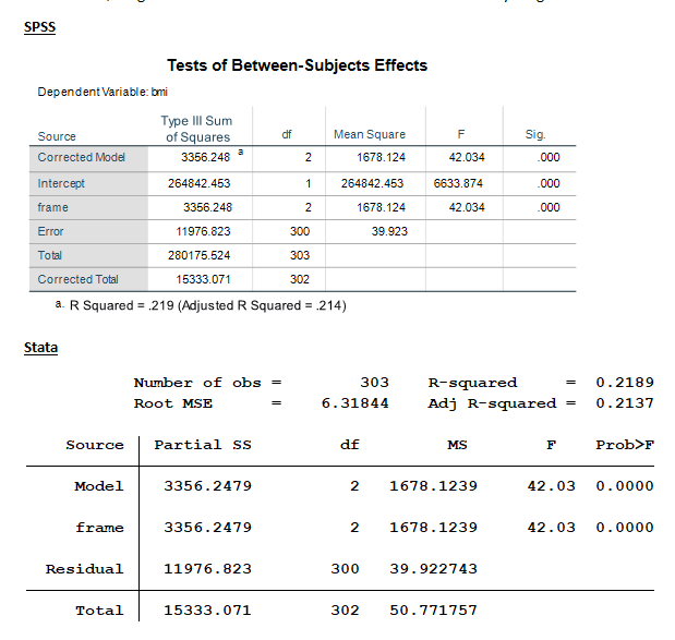
We could also have run this exact same model in an ANOVA procedure.  In SPSS this procedure is called UNIANOVA in syntax and General Linear Model in the menus. In Stata, it’s called just ANOVA.

When we do, we get the same numerical values as shown above but everything has different names.

All the numerical results shown in the Oneway models can be found in the ANOVA output. SPSS’ UNIANOVA model contains three additional calculations: Corrected Model, Intercept and Corrected Total. Note that “Total” for SPSS’S ANOVA model has a different meaning than the “Total” for the other three outputs.

Linear Regression Output

Stata’s linear regression procedure is once again slightly different. It does not include a separate main effect for frame, but only gives us the SS for the model as a whole.

An additional command must be used to generate the main effect. However, since this model contains only one predictor variable, the statistics that are here reported for Model are the exact same as we saw above for Frame. This wouldn’t work if we had more than one predictor in the model, but it does work in this simple example.

Unfortunately, I can’t show you SPSS’s linear regression output for this model.  Their linear regression model doesn’t allow a categorical (factor) predictor in the model. I would have had to custom dummy-code it myself.

A Comparison of Outputs

What are the similarities among the model outputs?

All five outputs provide us with the same values. Ultimately, we get an F statistic of 42.03 and its corresponding p-value.

If we work our way backward from the F, we find the same values in the MS (mean square) columns.

The df (degrees of freedom) are identical numerical values of 2, 300, and 302 across all outputs.

The same numerical values are found in the SS (sum of squares) columns.

The biggest difference is found in the names of the “source”. “Between Groups,” “Frame,” and “Model” have identical values, “Within Groups” and “Residuals” as well. Four out of the five models have identical values for “Total”.

What are degrees of freedom, sum of squares, mean squares and source? Stay tuned. Upcoming blog posts will define them and explain how they are incorporated into the modeling process.

Four Critical Steps in Building Linear Regression Models

While you’re worrying about which predictors to enter, you might be missing issues that have a big impact your analysis. This training will help you achieve more accurate results and a less-frustrating model building experience.

Take Me to The Video!