It’s really easy to mix up the concepts of association (as measured by correlation) and interaction. Or to assume if two variables interact, they must be associated. But it’s not actually true.
In statistics, they have different implications for the relationships among your variables. This is especially true when the variables you’re talking about are predictors in a regression or ANOVA model.
Association
Association between two variables means the values of one variable relate in some way to the values of the other. It is usually measured by correlation for two continuous variables and by cross tabulation and a Chi-square test for two categorical variables.
Unfortunately, there is no nice, descriptive measure for association between one categorical and one continuous variable. Point-biserial correlation works only if the categorical variable is binary. But either one-way analysis of variance or logistic regression can test an association (depending upon whether you think of the categorical variable as the independent or the dependent variable).
Essentially, association means the values of one variable generally co-occur with certain values of the other.
Interaction
Interaction is different. Whether two variables are associated says nothing about whether they interact in their effect on a third variable. Likewise, if two variables interact, they may or may not be associated.
An interaction between two variables means the effect of one of those variables on a third variable is not constant—the effect differs at different values of the other.
What Association and Interaction Describe in a Model
The following examples show three situations for three variables: X1, X2, and Y. X1 is a continuous independent variable, X2 is a categorical independent variable, and Y is the continuous dependent variable. I chose these types of variables to make the plots easy to read, but any of these variables could be either categorical or continuous.
Association without Interaction
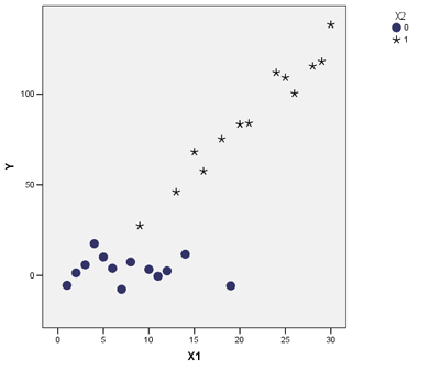
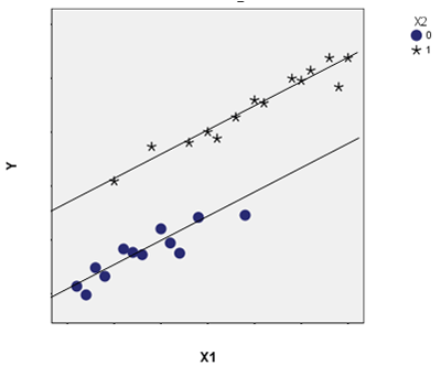
In scenario 1, X1 and X2 are associated. If you ignore Y, you can see the mean of X1 is lower when X2=0 than when X2=1. But they do not interact in how they affect Y—the regression lines are parallel. X1 has the same effect on Y (the slope) for both X2=1 and X2=0.
A simple example is the relationship between height (X1) and weight (Y) in male (X2=1) and female (X2=0) teenagers. There is a relationship between height (X1) and gender (X2). But for both genders, the relationship between height and weight is the same.
This is the situation you’re trying to take care of by including control variables. If you didn’t include gender as a control, a regression would fit a single line to all these points. It would attribute all variation in weights to differences in heights.
This line would also be steeper, as it tried to fit all the points using one line. As a result, it would overestimate the size of the unique effect of height on weight.
Interaction without Association
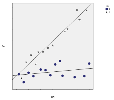
In a second scenario, X1 and X2 are not associated. The mean of X1 is the same for both categories of X2. But how X1 affects Y differs for the two values of X2. That’s the exact definition of an interaction. The slope of X1 on Y is greater for X2=1 than it is for X2=0, in which it is nearly flat.
An example of this would be an experiment in which X1 was a pretest score and Y a posttest score. Imagine you randomly assigned participants to a control (X2=1) or a training (X2=0) condition.
If randomization is done well, the assigned condition (X2) should be unrelated to the pretest score (X1). But they do interact—the relationship between pretest and posttest differs in the two conditions.
In the control condition, without training, the pretest and posttest scores would be highly correlated. But in the training condition, if the training worked well, pretest scores would have less effect on posttest scores.
Both Association and Interaction
In the third scenario, we’ve got both an association and an interaction. X1 and X2 are associated. Once again the mean of X1 is lower when X2=0 than when X2=1. They also interact with Y. The slopes of the relationship between X1 and Y are different when X2=0 and X2=1. So X2 affects the relationship between X1 and Y.
A good example here would be if Y is the number of jobs in a county, X1 is the percentage of the workforce that holds a college degree, and X2 is whether the county is rural (X2=0) or metropolitan (X2=1).
It’s clear rural counties have, on average, lower percentages of college-educated citizens than metropolitan counties. They also have fewer jobs.
It’s also clear that the workforce’s education level in metropolitan counties is related to how many jobs there are. But in rural counties, it doesn’t matter at all.
This situation is also what you would see if the randomization in the last example did not go well or if randomization was not possible.
 The differences between Interaction and Association will become clearer as you analyze more data. It’s always a good idea to stop and explore your data. Use graphs or try different terms in your model to figure out exactly what’s going on with your variables.
Go to the next article or see the full series on Easy-to-Confuse Statistical Concepts


Excelente texto elucidativo que esclarece de forma brilhante dois conceitos cuja comparação não se encontra acesso. Tema esquecido e muito bem abordado pela autora. Fico muito agradecido à esta sua idéia de tornar claro dois conceitos que são tratados na literatura estatísttica de forma separada .
I have a quick question about example #2.
Does it imply that the training actually hurt the posttest scores? If it helped, shouldn’t the regression line for X2=0 be pushed up, so that the average Y is higher?
Hi IC,
Yes, if high scores indicated improvement, that would be true. The whole line for the treatment group would be higher. But in many situations, “better” means “lower” like looking at frequency of errors or number of negative symptoms. I didn’t really specify either way.
Thanks Karen, in the examples you gave, what’s the difference between a model with interaction term and stratifying the model by different values of X2? Thank you.
Hi Steve,
I didn’t give an example with stratifying and I don’t generally recommend it. When you stratify, you’re running two separate models. There are multiple disadvanges–it’s statistically inefficient, meaning you end up with larger residual variance estimates and it no longer allows you to test the difference in coefficients for the two groups of X2.
Hi
Let me start by saying I’m not a mathematics expert. I need to know if there is a way to make the assumed factors weight which are randomly chosen based on experience effecting a decision making to assume that all of them are totally interacting (you call it here associated) and can we confirm their interaction by putting a test. Let’s say the test is the total sum for them will be 100% or equal 1.
Is the above is a known model what’s the name of it ?
Thanks a lot
Hi,
I have the following escenario:
-X is associated with Y
-Y is associated with Z
-X is not associated with Z
X and Y are categorical variables and Z is continuous.
How could I explain the no association between X and Z?
Thanks
Hi Tomas! Very interesting question! I will discuss a very similar case here, taken from Hayes (2013) – where M1 and M2 are two mediating variables between X (the independent variable) and Z (the dependent variable). That is, the effect of X on Z is through M1 and M2 (in other words, M1 and M2 are the pathways). It is possible that the indirect effect of X on Z through M1 is in a certain direction (say, positive), but the indirect effect through M2 is in the opposite direction (say, negative) but of equal magnitude. Then, the two indirect effects add up to zero, and if there is no other process at work linking X to Z, then the total effect will be zero, or there will be no correlation between X and Z.
In your case, it is possible that you are looking only at X, Z and M1 (which you have called as Y).
The above example is discussed in Hayes’ (2013) book. Please take a look at page 169 in the book.
Best of luck with your work!
Reference:
Hayes, A. F. (2013). Introduction to mediation, moderation, and conditional process analysis. (T. D. Little, Ed.). New York, NY: Guilford Press.
Hi, I wanted to show interaction between two independent(continuous ) variables for a dependent variable. The correlation between the variables is >0.6. Can i use enter both independent variables in regression if correlation is do high
Thanks for your very good article
Hi
I have the same question as Rekha.
Also would like to know if the correlation is 0.3 but statistically significant between the 2 variables.
I tested the interaction term in the model but it is not significant.
Could you please explain ?
Thanks
Theoretically, yes you can do it with correlated predictors. It should be fine with a correlation of .3, but .6 is pushing it.
In my last graph above, X1 and X2 are positively correlated, but the effects of X1 on Y are definitely different for the two groups of X2. So you have both correlation and interaction.
thanks a lot this helped a great deal
I think you meant “metropolitan (X2=1)” not “metropolitan (X1=0)”.
Thanks, JZ, I did! Just fixed it.
Thanks for clearly elaborating the difference between associations and interactions.
Can you please explain for me how to look for, and explain interactions when we have two independent categorical variables, say X1 (yes, no) and gender(male, female) with a categorical outcome say, Y(high, low)
Many thanks!
Hi Jonathan,
It basically comes down to: an interaction will occur in that case if the effect of a Yes for X1 has a different effect on the proportion of Highs in Y for each gender.
You have to be careful when your outcome is dichotomous.
In case of linear regression/ANOVA with continuous outcomes, interaction (or moderation of effect) is equal to departure from additivity.
In case of logistic regression with dichotomous outcome, interaction is equal to departure of multiplicity(!) of odds.
If you want to analyse interaction as departure from additivity of odds you have to do some tricks (see, Hosmer and Lemeshow, 1992, Epidemiology, 3, 452-456). This is sometimes called “biological interaction” (see, Rothman & Greenland, 1998, Modern Epidemiology, 2nd ed., Chap. 18).
Hi Wobbe,
Agreed, odds ratios are already on a multiplicative scale.
And we do this to make interpretation of coefficients easier. What I wrote does hold even in logistic regression for the coefficients themselves, which measure differences, not ratios.