So, you want to get started with Stata?
Good choice!
At The Analysis Factor we recommend first becoming proficient in one statistical software. Then once you’ve progressed up to learning Stage 3 skills, adding a second statistical software. Whether it’s your first, second, or 5th statistical software, Stata has a lot that makes it worth learning.
When I first started using Stata, I remember being confused by the variety of menus and windows, the strange syntax of the code, the way it handled datasets… and what the heck is a do file?
In this blog post, I want to get you started with Stata from the very beginning – working with Stata’s windows. We have a lot of great resources on more advanced Stata topics, but it’s important to nail down the basics first.
When I started using Stata, I wanted to skip the hour or so it would take to nail down the details of the software so I could go straight into making the regression that I needed for my class. Skipping the basics at the beginning cost me hours of hardship later on as I struggled to understand the structure of Stata.
I was also never told how easy Stata makes it to get help.
So – from the beginning.
You need to download the software. You can purchase and download Stata from https://www.stata.com/.
Stata is not free, but it is reasonably priced for all that you get, generally lower than SAS or SPSS. Pricing varies by institution (students and educators get discounts), length of the license, and the processing power you choose to request. After purchasing you should receive via email a license key to run the software.
Once you’ve done all that, you should open the program. You will see five windows and a variety of icons and menus. This is a lot to process, so let’s break it down one piece at a time.
Stata’s Windows
We have the following windows: History, Results, Command, Variables, and Properties.
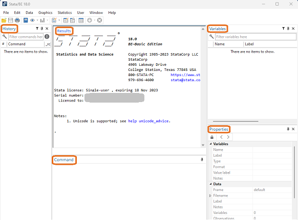
You can move, resize, or pin any of these windows .
The Command Window
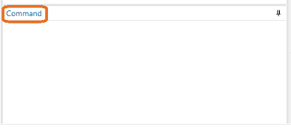 In Stata you use the Command Window to enter commands. Start by typing the following into the command line, then press enter.
sysuse auto
This command tells Stata to load up the auto dataset, one of the ones installed in the software by default.
Stata only allows one dataset to be open at a time. This means you can easily refer to variable names without specifying which dataset they come from.
We can now run a regression on two of these variables by typing:
regress price mpg
or
reg price mpg
and then pressing enter.
This tells Stata to regress price on mpg and output the results. You can see here that Stata allows shorthand forms of certain commands.
Each time you enter a command in the Command Window, the words you typed as well as any associated output will appear in the Results Window.
The Results Window
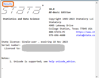 Whenever Stata runs code, either through the command line or a do file, the Results Window will hold all the output. This is the place you will look right after running a command or do-file.
We can also use the Results Window to export our output.
Try highlighting the regression table and see the options “copy table” and “copy as picture”. These options allow you to put regression output or other results into a document or spreadsheet.
The History Window
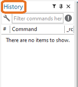 To the left of your screen lies the History Window. This contains a list of every command you’ve entered in the current Stata session.
If you want to redo a command you previously typed, simply click on that code in your history and it will appear in your Command Window, where you can edit it or enter it as-is.
Once you get to using do-files, the History Window will keep track of which do files you have run. Even better, you can use it to rerun those files.
You can use the search bar in the History Window to find a particular command you previously entered.
The Variable Window
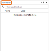 Once we have a dataset, the Variables Window will list all variables in the dataset, as well as each of their labels.
As we hover over a variable, a downward arrow appears to the left of the name. Clicking this arrow or double clicking the variable immediately pastes the variable name into the
Command Window.
So you can type
reg
Then double click on price, then on mpg. Notice how the command is the same as the one you had typed.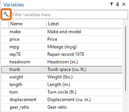
With the wrench icon on the top left, you can filter variables or change the display in the column tab.
As you click on each variable name, notice how the Properties Window changes what it displays.
The Properties Window
As you select a variable from the variables list, its details will show up in the Properties Window.
This window displays the name, label, type, format, value label, and notes of a given variable (if these exist).
Below this we see information about the dataset in general including the file name, label, size, number of observations, and more.
In the top left of the Properties Window, we see a lock symbol. If we click this to unlock it, we can now change features of our dataset.
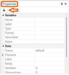 Click on the gear_ratio variable in the Variables Window, then click the lock in the Properties Window.
Notice how you can now change the name, label and more? Try renaming the length variable to “gear_rat” and press enter. You will see this output in the results window:
rename gear_ratio gear_rat
We see here that when you use menus to make changes to the dataset or run analysis, Stata also puts the same commands into the Results Window. This makes it easy to learn code by doing things first in the menus.
If we want to change the name back to how it was before, you could change it through the menus, or type
rename gear_rat gear_ratio
And just like that, you’re a master of navigating windows in Stata.
by James Harrod
About the Author: James Harrod interned at The Analysis Factor in the summer of 2023. He plans to continue into a career as an actuary, and hopes to continue finding interesting ways of educating people about statistics. James is well-versed in R and Stata programming and enjoys teaching the intuition behind common statistical methods. James is a 2023 graduate of the University of Rochester with bachelor’s degrees in Statistics and Economics.


Leave a Reply