A number of years ago when I was still working in the consulting office at Cornell, someone came in asking for help interpreting their ordinal logistic regression results.
The client was surprised because all the coefficients were backwards from what they expected, and they wanted to make sure they were interpreting them correctly.
It looked like the researcher had done everything correctly, but the results were definitely bizarre. They were using SPSS and the manual wasn’t clarifying anything for me, so I did the logical thing: I ran it in another software program. I wanted to make sure the problem was with interpretation, and not in some strange default or (more…)
One of the nice features of SPSS is its ability to keep track of information on the variables themselves.

This includes variable labels, missing data codes, value labels, and variable formats. Spending the time to set up variable information makes data analysis much easier–you don’t have to keep looking up whether males are coded 1 or 0, for example.
And having them all in the variable view window makes things incredibly easy while you’re doing your analysis. But sometimes you need to just print them all out–to create a code book for another analyst or to include in the output you’re sending to a collaborator. Or even just to print them out for yourself for easy reference.
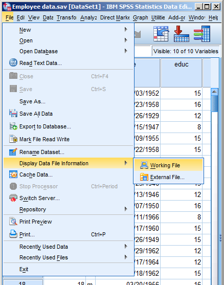
There is a nice little way to get a few tables with a list of all the variable metadata. It’s in the File menu. Simply choose Display Data File Information and Working File.
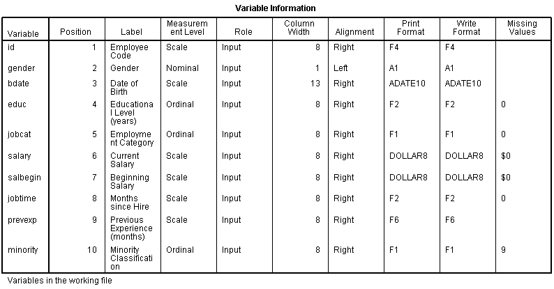
Doing this gives you two tables. The first includes the following information on the variables. I find the information I use the most are the labels and the missing data codes.


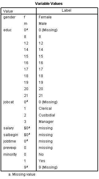
Even more useful, though, is the Value Label table.
It lists out the labels for all the values for each variable.
So you don’t have to remember that Job Category (jobcat) 1 is “Clerical,” 2 is “Custodial,” and 3 is “Managerial.”
It’s all right there.
Two methods for dealing with missing data, vast improvements over traditional approaches, have become available in mainstream statistical software in the last few years.
Both of the methods discussed here require that the data are missing at random–not related to the missing values. If this assumption holds, resulting estimates (i.e., regression coefficients and standard errors) will be unbiased with no loss of power.
The first method is Multiple Imputation (MI). Just like the old-fashioned imputation (more…)
Before you run a Cronbach’s alpha or factor analysis on scale items, it’s generally a good idea to reverse code items that are negatively worded so that a high value indicates the same type of response on every item.
So for example let’s say you have 20 items each on a 1 to 7 scale. For most items, a 7 may indicate a positive attitude toward some issue, but for a few items, a 1 indicates a positive attitude.
I want to show you a very quick and easy way to reverse code them using a single command line. This works in any software. (more…)
It seems every editor and her brother these days wants to see standardized effect size statistics reported in journal articles.
For ANOVAs, two of the most popular are Eta-squared and partial Eta-squared. In one way ANOVAs, they come out the same, but in more complicated models, their values, and their meanings differ.
SPSS only reports partial Eta-squared, and in earlier versions of the software it was (unfortunately) labeled Eta-squared. More recent versions have fixed the label, but still don’t offer Eta-squared as an option.
Luckily Eta-squared is very simple to calculate yourself based on the sums of squares in your ANOVA table. I’ve written another blog post with all the formulas. You can (more…)
In my last blog post, I wrote about a mistake I once made when I didn’t realize the defaults for dummy coding were different in two SPSS procedures (Binary Logistic and GEE).
Ironically, about the same time I wrote it, I was having a conversation with Ann Maria de Mars on Twitter. She was trying to figure out why her logistic regression model fit results were identical in SAS Proc Logistic and SPSS Binary Logistic, but the coefficients in SAS were half those of SPSS.
It was ironic because I, of course, didn’t recognize it as the same issue and wasn’t much help.
But Ann Maria investigated and discovered that it came down to differences in the defaults for coding categorical predictors in SAS and SPSS that did it. Her detailed and humorous explanation is here.
Some takeaways for you, the researcher and data analyst:
1. Give yourself a break if you hit a snag. Even very experienced data analysts, statisticians who understand what they’re doing, get stumped sometimes. Don’t ever think that performing data analysis is an IQ test. You’re bringing together many skills and complex tools.
2. Learn thy software. In my last post, I phrased it “Know thy software”, but this is where you get to know it. Snags are good opportunities to investigate the details of your software, just like Ann Maria did. If you can think of it as a challenge to figure out–a puzzle–it can actually be fun.
Make friends with your syntax manuals.
3. Get help when you need it. Statistical software packages *are* complex tools. You don’t have to know everything to use them
Ask colleagues. Call customer support. Call a stat consultant. That’s what they’re there for.
4. A great way to check your work is to run your test two different ways. It’s another reason to be able to use at least two stat software packages. I’m not suggesting you have to run every analysis twice. But when a result looks strange, or you want to double-check a specific important model, this can be a good strategy for testing things out.
It may be that your results aren’t telling you what you think they are.
[Logistic_Regression_Workshop]

