In a previous article, we discussed how incidence rate ratios calculated in a Poisson regression can be determined from a two-way table of categorical variables.
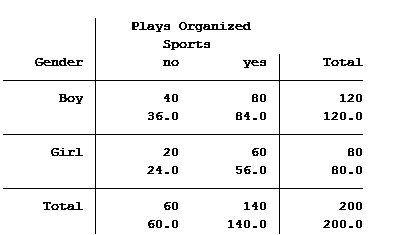
Statistical software can also calculate the expected (aka predicted) count for each group. Below is the actual and expected count of the number of boys and girls participating and not participating in organized sports.

The value in the top of each cell is the actual count (40 boys do not play organized sports) and the bottom value is the expected/predicted count (36 boys are predicted to not play organized sports).
The Poisson model that we ran in the previous article generated the following table: (more…)
The coefficients of count model regression tables are shown in either logged form or as incidence rate ratios. Trying to explain the coefficients in logged form can be a difficult process.
Incidence rate ratios are much easier to explain. You probably didn’t realize you’ve seen incidence rate ratios before, expressed differently.
Let’s look at an example.
A school district was interested in how many children in their sixth grade classes played on organized sports teams. So they did a count and also noted the gender of the child. The results were put into a table: (more…)
The normal distribution is so ubiquitous in statistics that those of us who use a lot of statistics tend to forget it’s not always so common in actual data.
And since the normal distribution is continuous, many people describe all numerical variables as continuous. I get it: I’m guilty of using those terms interchangeably, too, but they’re not exactly the same.
Numerical variables can be either continuous or discrete.
The difference? Continuous variables can take any number within a range. Discrete variables can only take on specific values. For numeric discrete data, these are often, but don’t have to be, whole numbers*.
Count variables, as the name implies, are frequencies of some event or state. Number of arrests, fish (more…)
If you have count data you use a Poisson model for the analysis, right?
The key criterion for using a Poisson model is after accounting for the effect of predictors, the mean must equal the variance. If the mean doesn’t equal the variance then all we have to do is transform the data or tweak the model, correct?
Let’s see how we can do this with some real data. A survey was done in Australia during the peak of the flu season. The outcome variable is the total number of times people asked for medical advice from any source over a two-week period.
We are trying to determine what influences people with flu symptoms to seek medical advice. The mean number of times was 0.516 times and the variance 1.79.
The mean does not equal the variance even after accounting for the model’s predictors.
Here are the results for this model: (more…)
A common situation with count outcome variables is there are a lot of zero values. The Poisson distribution used for modeling count variables takes into account that zeros are often the most

common value, but sometimes there are even more zeros than the Poisson distribution can account for.
This can happen in continuous variables as well–most of the distribution follows a beautiful normal distribution, except for the big stack of zeros.
This webinar will explore two ways of modeling zero-inflated data: the Zero Inflated model and the Hurdle model. Both assume there are two different processes: one that affects the probability of a zero and one that affects the actual values, and both allow different sets of predictors for each process.
We’ll explore these models as well as some related models, like Zero-One Inflated Beta models for proportion data.
Note: This training is an exclusive benefit to members of the Statistically Speaking Membership Program and part of the Stat’s Amore Trainings Series. Each Stat’s Amore Training is approximately 90 minutes long.
(more…)
In a previous post we explored bounded variables and the difference between truncated and censored. Can we ignore the fact that a variable is bounded and just run our analysis as if the data wasn’t bounded? (more…)


