Have you ever been told you need to run a mixed (aka: multilevel) model and been thrown off by all the new vocabulary?
It happened to me when I first started my statistical consulting job, oh so many years ago. I had learned mixed models in an ANOVA class, so I had a pretty good grasp on many of the concepts.
But when I started my job, SAS had just recently come out with Proc Mixed, and it was the first time I had to actually implement a true multilevel model. I was out of school, so I had to figure it out on the job.
And even with my background, I had a pretty steep learning curve to get to a point where it made sense. Sure, I was able to figure out the steps, but there are some pretty tricky situations and complicated designs out there.
To implement it well, you need a good understanding of the big picture, and how the small parts fit into it. (more…)

In Part 2 of this series, we created two variables and used the lm() command to perform a least squares regression on them, treating one of them as the dependent variable and the other as the independent variable. Here they are again.
height = c(176, 154, 138, 196, 132, 176, 181, 169, 150, 175)
bodymass = c(82, 49, 53, 112, 47, 69, 77, 71, 62, 78)
Today we learn how to obtain useful diagnostic information about a regression model and then how to draw residuals on a plot. As before, we perform the regression.
lm(height ~ bodymass)
Call:
lm(formula = height ~ bodymass)
Coefficients:
(Intercept) bodymass
98.0054 0.9528
Now let’s find out more about the regression. First, let’s store the regression model as an object called mod and then use the summary() command to learn about the regression.
mod <- lm(height ~ bodymass)
summary(mod)
Here is what R gives you.
Call:
lm(formula = height ~ bodymass)
Residuals:
Min 1Q Median 3Q Max
-10.786 -8.307 1.272 7.818 12.253
Coefficients:
Estimate Std. Error t value Pr(>|t|)
(Intercept) 98.0054 11.7053 8.373 3.14e-05 ***
bodymass 0.9528 0.1618 5.889 0.000366 ***
Signif. codes: 0 ‘***’ 0.001 ‘**’ 0.01 ‘*’ 0.05 ‘.’ 0.1 ‘ ’ 1
Residual standard error: 9.358 on 8 degrees of freedom
Multiple R-squared: 0.8126, Adjusted R-squared: 0.7891
F-statistic: 34.68 on 1 and 8 DF, p-value: 0.0003662
R has given you a great deal of diagnostic information about the regression. The most useful of this information are the coefficients themselves, the Adjusted R-squared, the F-statistic and the p-value for the model.
Now let’s use R’s predict() command to create a vector of fitted values.
regmodel <- predict(lm(height ~ bodymass))
regmodel
Here are the fitted values:
1 2 3 4 5 6 7 8 9 10
176.1334 144.6916 148.5027 204.7167 142.7861 163.7472 171.3695 165.6528 157.0778 172.3222
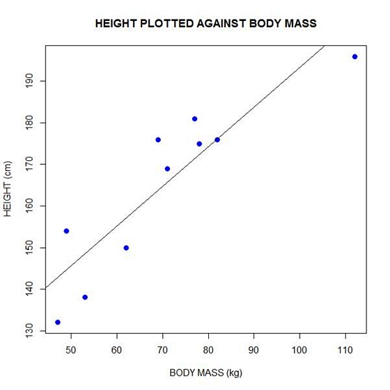
Now let’s plot the data and regression line again.
plot(bodymass, height, pch = 16, cex = 1.3, col = "blue", main = "HEIGHT PLOTTED AGAINST BODY MASS", xlab = "BODY MASS (kg)", ylab = "HEIGHT (cm)")
abline(lm(height ~ bodymass))
We can plot the residuals using R’s for loop and a subscript k that runs from 1 to the number of data points. We know that there are 10 data points, but if we do not know the number of data we can find it using the length() command on either the height or body mass variable.
npoints <- length(height)

npoints
[1] 10
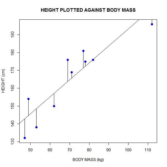
Now let’s implement the loop and draw the residuals (the differences between the observed data and the corresponding fitted values) using the lines() command. Note the syntax we use to draw in the residuals.
for (k in 1: npoints) lines(c(bodymass[k], bodymass[k]), c(height[k], regmodel[k]))
Here is our plot, including the residuals.
In part 4 we will look at more advanced aspects of regression models and see what R has to offer.
About the Author: David Lillis has taught R to many researchers and statisticians. His company, Sigma Statistics and Research Limited, provides both on-line instruction and face-to-face workshops on R, and coding services in R. David holds a doctorate in applied statistics.
See our full R Tutorial Series and other blog posts regarding R programming.
Standardized regression coefficients remove the unit of measurement of predictor and outcome variables. They are sometimes called betas, but I don’t like to use that term because there are too many other, and too many related, concepts that are also called beta.
There are many good reasons to report them:
- They serve as standardized effect size statistics.
- They allow you to compare the relative effects of predictors measured on different scales.
- They make journal editors and committee members happy in fields where they are commonly reported. (more…)
I received an e-mail from a researcher in Canada that asked about communicating logistic regression results to non-researchers. It was an important question, and there are a number of parts to it.
With the asker’s permission, I am going to address it here.
To give you the full context, she explained in a follow-up email that she is communicating to a clinical audience who will be using the results to make clinical decisions. They need to understand the size of an effect that an intervention will provide. She refers to an output I presented in my webinar on Probability, Odds, and Odds Ratios, which you can view free here.
Question:
I just went through the two lectures re: logistic regression and prob/odds/odds ratios. I completely understand (more…)
Every once in a while, I work with a client who is stuck between a particular statistical rock and hard place. It happens when they’re trying to run an analysis of covariance (ANCOVA) model because they have a categorical independent variable and a continuous covariate.

The problem arises when a coauthor, committee member, or reviewer insists that ANCOVA is inappropriate in this situation because one of the following ANCOVA assumptions are not met:
1. The independent variable and the covariate are independent of each other.
2. There is no interaction between independent variable and the covariate.
If you look them up in any design of experiments textbook, which is usually where you’ll find information about ANOVA and ANCOVA, you will indeed find these assumptions. So the critic has nice references.
However, this is a case where it’s important to stop and think about whether the assumptions apply to your situation, and how dealing with the assumption will affect the analysis and the conclusions you can draw. (more…)
When the response variable for a regression model is categorical, linear models don’t work. Logistic regression is one type of model that does, and it’s relatively straightforward for binary responses.
When the response variable is not just categorical, but ordered categories, the model needs to be able to handle the multiple categories, and ideally, account for the ordering.
An easy-to-understand and common example is level of educational attainment. Depending on the population being studied, some response categories may include:
1 Less than high school
2 Some high school, but no degree
3 Attain GED
4 High school graduate
You can see how there are qualitative differences in these categories that wouldn’t be captured by years of education. You can also see that (more…)