Linear Regression

Interpreting Regression Coefficients: Changing the scale of predictor variables

October 11th, 2021 by

One issue that affects how to interpret regression coefficients is the scale of the variables. In linear regression, the scaling of both the response variable Y, and the relevant predictor X, are both important.

In regression models like logistic regression, where the response variable is categorical, and therefore doesn’t have a numerical scale, this only applies to predictor variables, X.

This can be an issue of measurement units–miles vs. kilometers. Or it can be an issue of simply how big “one unit” is. For example, whether one unit of annual income is measured in dollars, thousands of dollars, or millions of dollars.

The good news is you can easily change the scale of variables to make it easier to interpret their regression coefficients. This works as well for functions of regression coefficients, like odds ratios and rate ratios.

All you have to do is create a new variable in your data set (don’t overwrite the individual one in case you make a mistake). This new variable is simply the old one multiplied or divided by some constant.  The constant is often a factor of 10, but it doesn’t have to be. Then use the new variable in your model instead of the original one.

Since regression coefficients and odds ratios tell you the effect of a one unit change in the predictor, you should multiply them so that a one unit change in the predictor makes sense.

An Example of Rescaling Predictors

Here is a really simple example that I use in one of my workshops.

Y= first semester college GPA

X1= high school GPA
X2=SAT score

High School and first semester College GPA are both measured on a scale from 0 to  4. If you’re not familiar with this scaling, a 0 means you failed a class. An A (usually the top possible score) is a 4, a B is a 3, a C is a 2, and a D is a 1. So for a grade point average, a one point difference is very big.

If you’re an admissions counselor looking at high school transcripts, there is a big difference between a 3.7 GPA and a 2.7 GPA.

SAT score is on an entirely different scale. It’s a normed scale, so that the minimum is 200, the maximum is 800, and the mean is 500. Scores are in units of 10. You literally cannot receive a score of 622. You can get only 620 or 630.

So a one-point difference is not only tiny, it’s meaningless. Even a 10 point difference in SAT scores is pretty small. But 50 points is meaningful, and 100 points is large.

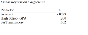
If you leave both predictors on the original scale in a regression that predicts first semester GPA, you get the following results:

Let’s interpret those coefficients.

The coefficient for high school GPA here is .20. This says that for each one-unit difference in GPA, we expect, on average, a .2 higher first semester GPA. While a one-unit change in GPA is huge, that’s reasonably meaningful.

The coefficient for SAT math scores is .002. That looks tiny. It says that for each one-unit difference in SAT math score, we expect, on average, a .002 higher first semester GPA. But a one-unit difference in SAT score is too small to interpret. It’s too small to be meaningful.

So we can change the scaling of our SAT score predictor to be in 10-point differences. Or in 100 point differences. Chose the scale for which one unit is meaningful.

Changing the scale by mulitplying the coefficient

In a linear model, you can simply multiply the coefficient by 10 to reflect a 10-point difference. That’s a coefficient of .02. So for each 10 point difference in math SAT score we expect, on average, a .02 higher first semester GPA.

Or we could multiply the coefficient by 50 to reflect a 50-point difference. That’s a coefficient of .10. So for each 50 point difference in math SAT score we expect, on average, a .1 higher first semester GPA.

When it’s easier to just change the variables

Multiplying the coefficient is easier than rescaling the original variable if you only have one or two of these and you’re using linear regression.

It doesn’t work once you’ve done any sort of back-transformation in generalized linear models. So you can’t just multiply the odds ratio or the incidence rate ratio by 10 or 50. Both of these are created by exponentiating the regression coefficient. Because of the order of operations in algebra, You have to first multiply the coefficient by the constant, and then re-expontiate.

Likewise, if you are using this predictor in more than one linear regression model, it’s much simpler to rescale the variable in the first place. Simply divide that SAT score by 10 or 50 and the coefficient will .02 or .10, respectively.

Updated 12/2/2021


Member Training: Matrix Algebra for Data Analysts: A Primer

August 31st, 2021 by

If you’ve been doing data analysis for very long, you’ve certainly come across terms, concepts, and processes of matrix algebra.  Not just matrices, but:

  • Matrix addition and multiplication
  • Traces and determinants
  • Eigenvalues and Eigenvectors
  • Inverting and transposing
  • Positive and negative definite

(more…)


Centering a Covariate to Improve Interpretability

April 9th, 2021 by

Centering a covariate –a continuous predictor variable–can make regression coefficients much more interpretable. That’s a big advantage, particularly when you have many coefficients to interpret. Or when you’ve included terms that are tricky to interpret, like interactions or quadratic terms.

For example, say you had one categorical predictor with 4 categories and one continuous covariate, plus an interaction between them.

First, you’ll notice that if you center your covariate at the mean, there is (more…)


Member Training: Statistical Contrasts

March 31st, 2021 by


Statistical contrasts are a tool for testing specific hypotheses and model effects, particularly comparing specific group means.

(more…)


Member Training: Goodness of Fit Statistics

March 4th, 2021 by


What are goodness of fit statistics? Is the definition the same for all types of statistical model? Do we run the same tests for all types of statistic model?

(more…)


Confusing Statistical Term #9: Multiple Regression Model and Multivariate Regression Model

February 20th, 2021 by

Much like General Linear Model and Generalized Linear Model in #7, there are many examples in statistics of terms with (ridiculously) similar names, but nuanced meanings.
Stage 2

Today I talk about the difference between multivariate and multiple, as they relate to regression.

Multiple Regression

A regression analysis with one dependent variable and eight independent variables is NOT a multivariate regression model.  It’s a multiple regression model.

And believe it or not, it’s considered a univariate model.

This is uniquely important to remember if you’re an SPSS user. Choose Univariate GLM (General Linear Model) for this model, not multivariate.

I know this sounds crazy and misleading because why would a model that contains nine variables (eight Xs and one Y) be considered a univariate model?

It’s because of the fundamental idea in regression that Xs and Ys aren’t the same. We’re using the Xs to understand the mean and variance of Y. This is why the residuals in a linear regression are differences between predicted and actual values of Y. Not X.

(And of course, there is an exception, called Type II or Major Axis linear regression, where X and Y are not distinct. But in most regression models, Y has a different role than X).

It’s the number of Ys that tell you whether it’s a univariate or multivariate model. That said, other than SPSS, I haven’t seen anyone use the term univariate to refer to this model in practice. Instead, the assumed default is that indeed, regression models have one Y, so let’s focus on how many Xs the model has. This leads us to…

Simple Regression: A regression model with one Y (dependent variable) and one X (independent variable).

Multiple Regression: A regression model with one Y (dependent variable) and more than one X (independent variables).

References below.

Multivariate Regression

Multivariate analysis ALWAYS describes a situation with multiple dependent variables.

So a multivariate regression model is one with multiple Y variables. It may have one or more than one X variables. It is equivalent to a MANOVA: Multivariate Analysis of Variance.

Other examples of Multivariate Analysis include:

  • Principal Component Analysis
  • Factor Analysis
  • Canonical Correlation Analysis
  • Linear Discriminant Analysis
  • Cluster Analysis

But wait. Multivariate analyses like cluster analysis and factor analysis have no dependent variable, per se. Why is it about dependent variables?

Well,  it’s not really about dependency.  It’s about which variables’ mean and variance is being analyzed.  In a multivariate regression, we have multiple dependent variables, whose joint mean is being predicted by the one or more Xs. It’s the variance and covariance in the set of Ys that we’re modeling (and estimating in the Variance-Covariance matrix).

Note: this is actually a situation where the subtle differences in what we call that Y variable can help.  Calling it the outcome or response variable, rather than dependent, is more applicable to something like factor analysis.

So when to choose multivariate GLM?  When you’re jointly modeling the variation in multiple response variables.

References

In response to many requests in the comments, I suggest the following references.  I give the caveat, though, that neither reference compares the two terms directly. They simply define each one. So rather than just list references, I’m going to explain them a little.

  1. Neter, Kutner, Nachtsheim, Wasserman’s Applied Linear Regression Models, 3rd ed. There are, incidentally, newer editions with slight changes in authorship. But I’m citing the one on my shelf.

Chapter 1, Linear Regression with One Independent Variable, includes:

“Regression model 1.1 … is “simple” in that there is only one predictor variable.”

Chapter 6 is titled Multiple Regression – I, and section 6.1 is “Multiple Regression Models: Need for Several Predictor Variables.” Interestingly enough, there is no direct quotable definition of the term “multiple regression.” Even so, it’s pretty clear. Go read the chapter to see.

There is no mention of the term “Multivariate Regression” in this book.

2. Johnson & Wichern’s Applied Multivariate Statistical Analysis, 3rd ed.

Chapter 7, Multivariate Linear Regression Models, section 7.1 Introduction. Here it says:

“In this chapter we first discuss the multiple regression model for the prediction of a single response. This model is then generalized to handle the prediction of several dependent variables.” (Emphasis theirs).

They finally get to Multivariate Multiple Regression in Section 7.7. Here they “consider the problem of modeling the relationship between m responses, Y1, Y2, …,Ym, and a single set of predictor variables.”

Misuses of the Terms

I’d be shocked, however, if there aren’t some books or articles out there where the terms are not used or defined  the way I’ve described them here, according to these references. It’s very easy to confuse these terms, even for those of us who should know better.

And honestly, it’s not that hard to just describe the model instead of naming it. “Regression model with four predictors and one outcome” doesn’t take a lot more words and is much less confusing.

If you’re ever confused about the type of model someone is describing to you, just ask.

Read More Explanations of Confusing Statistical Terms.

First Published 4/29/09;
Updated 2/23/21 to give more detail.