Linear, Logistic, Tobit, Cox, Poisson, Zero Inflated… The list of regression models goes on and on before you even get to things like ANCOVA or Linear Mixed Models.
In this webinar, we will explore types of regression models, how they differ, how they’re the same, and most importantly, when to use each one.
Note: This training is an exclusive benefit to members of the Statistically Speaking Membership Program and part of the Stat’s Amore Trainings Series. Each Stat’s Amore Training is approximately 90 minutes long.
About the Instructor

Karen Grace-Martin helps statistics practitioners gain an intuitive understanding of how statistics is applied to real data in research studies.
She has guided and trained researchers through their statistical analysis for over 15 years as a statistical consultant at Cornell University and through The Analysis Factor. She has master’s degrees in both applied statistics and social psychology and is an expert in SPSS and SAS.
Not a Member Yet?
It’s never too early to set yourself up for successful analysis with support and training from expert statisticians.
Just head over and sign up for Statistically Speaking.
You'll get access to this training webinar, 130+ other stats trainings, a pathway to work through the trainings that you need — plus the expert guidance you need to build statistical skill with live Q&A sessions and an ask-a-mentor forum.

In Part 2 of this series, we created two variables and used the lm() command to perform a least squares regression on them, treating one of them as the dependent variable and the other as the independent variable. Here they are again.
height = c(176, 154, 138, 196, 132, 176, 181, 169, 150, 175)
bodymass = c(82, 49, 53, 112, 47, 69, 77, 71, 62, 78)
Today we learn how to obtain useful diagnostic information about a regression model and then how to draw residuals on a plot. As before, we perform the regression.
lm(height ~ bodymass)
Call:
lm(formula = height ~ bodymass)
Coefficients:
(Intercept) bodymass
98.0054 0.9528
Now let’s find out more about the regression. First, let’s store the regression model as an object called mod and then use the summary() command to learn about the regression.
mod <- lm(height ~ bodymass)
summary(mod)
Here is what R gives you.
Call:
lm(formula = height ~ bodymass)
Residuals:
Min 1Q Median 3Q Max
-10.786 -8.307 1.272 7.818 12.253
Coefficients:
Estimate Std. Error t value Pr(>|t|)
(Intercept) 98.0054 11.7053 8.373 3.14e-05 ***
bodymass 0.9528 0.1618 5.889 0.000366 ***
Signif. codes: 0 ‘***’ 0.001 ‘**’ 0.01 ‘*’ 0.05 ‘.’ 0.1 ‘ ’ 1
Residual standard error: 9.358 on 8 degrees of freedom
Multiple R-squared: 0.8126, Adjusted R-squared: 0.7891
F-statistic: 34.68 on 1 and 8 DF, p-value: 0.0003662
R has given you a great deal of diagnostic information about the regression. The most useful of this information are the coefficients themselves, the Adjusted R-squared, the F-statistic and the p-value for the model.
Now let’s use R’s predict() command to create a vector of fitted values.
regmodel <- predict(lm(height ~ bodymass))
regmodel
Here are the fitted values:
1 2 3 4 5 6 7 8 9 10
176.1334 144.6916 148.5027 204.7167 142.7861 163.7472 171.3695 165.6528 157.0778 172.3222
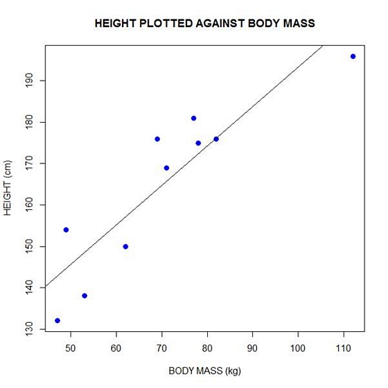
Now let’s plot the data and regression line again.
plot(bodymass, height, pch = 16, cex = 1.3, col = "blue", main = "HEIGHT PLOTTED AGAINST BODY MASS", xlab = "BODY MASS (kg)", ylab = "HEIGHT (cm)")
abline(lm(height ~ bodymass))

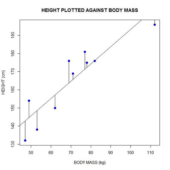
We can plot the residuals using R’s for loop and a subscript k that runs from 1 to the number of data points. We know that there are 10 data points, but if we do not know the number of data we can find it using the length() command on either the height or body mass variable.
npoints <- length(height)

npoints
[1] 10
Now let’s implement the loop and draw the residuals (the differences between the observed data and the corresponding fitted values) using the lines() command. Note the syntax we use to draw in the residuals.
for (k in 1: npoints) lines(c(bodymass[k], bodymass[k]), c(height[k], regmodel[k]))
Here is our plot, including the residuals.

In part 4 we will look at more advanced aspects of regression models and see what R has to offer.
About the Author: David Lillis has taught R to many researchers and statisticians. His company, Sigma Statistics and Research Limited, provides both on-line instruction and face-to-face workshops on R, and coding services in R. David holds a doctorate in applied statistics.
See our full R Tutorial Series and other blog posts regarding R programming.
Standardized regression coefficients remove the unit of measurement of predictor and outcome variables. They are sometimes called betas, but I don’t like to use that term because there are too many other, and too many related, concepts that are also called beta.
There are many good reasons to report them:
- They serve as standardized effect size statistics.
- They allow you to compare the relative effects of predictors measured on different scales.
- They make journal editors and committee members happy in fields where they are commonly reported. (more…)
Every once in a while, I work with a client who is stuck between a particular statistical rock and hard place. It happens when they’re trying to run an analysis of covariance (ANCOVA) model because they have a categorical independent variable and a continuous covariate.

The problem arises when a coauthor, committee member, or reviewer insists that ANCOVA is inappropriate in this situation because one of the following ANCOVA assumptions are not met:
1. The independent variable and the covariate are independent of each other.
2. There is no interaction between independent variable and the covariate.
If you look them up in any design of experiments textbook, which is usually where you’ll find information about ANOVA and ANCOVA, you will indeed find these assumptions. So the critic has nice references.
However, this is a case where it’s important to stop and think about whether the assumptions apply to your situation, and how dealing with the assumption will affect the analysis and the conclusions you can draw. (more…)
Like some of the other terms in our list–level and beta–GLM has two different meanings.
It’s a little different than the others, though, because it’s an abbreviation for two different terms:
General Linear Model and Generalized Linear Model.
It’s extra confusing because their names are so similar on top of having the same abbreviation.
And, oh yeah, Generalized Linear Models are an extension of General Linear Models.
And neither should be confused with Generalized Linear Mixed Models, abbreviated GLMM.
Naturally. (more…)
I am reviewing your notes from your workshop on assumptions. You have made it very clear how to analyze normality for regressions, but I could not find how to determine normality for ANOVAs. Do I check for normality for each independent variable separately? Where do I get the residuals? What plots do I run? Thank you!
I received this great question this morning from a past participant in my Assumptions of Linear Models workshop.
It’s one of those quick questions without a quick answer. Or rather, without a quick and useful answer. The quick answer is:
Do it exactly the same way. All of it.
The longer, useful answer is this: (more…)

