
In Part 3 we used the lm() command to perform least squares regressions. In Part 4 we will look at more advanced aspects of regression models and see what R has to offer.
One way of checking for non-linearity in your data is to fit a polynomial model and check whether the polynomial model fits the data better than a linear model. However, you may also wish to fit a quadratic or higher model because you have reason to believe that the relationship between the variables is inherently polynomial in nature. Let’s see how to fit a quadratic model in R.
We will use a data set of counts of a variable that is decreasing over time. Cut and paste the following data into your R workspace.
A <- structure(list(Time = c(0, 1, 2, 4, 6, 8, 9, 10, 11, 12, 13,
14, 15, 16, 18, 19, 20, 21, 22, 24, 25, 26, 27, 28, 29, 30),
Counts = c(126.6, 101.8, 71.6, 101.6, 68.1, 62.9, 45.5, 41.9,
46.3, 34.1, 38.2, 41.7, 24.7, 41.5, 36.6, 19.6,
22.8, 29.6, 23.5, 15.3, 13.4, 26.8, 9.8, 18.8, 25.9, 19.3)), .Names = c("Time", "Counts"),
row.names = c(1L, 2L, 3L, 5L, 7L, 9L, 10L, 11L, 12L, 13L, 14L, 15L, 16L, 17L, 19L, 20L, 21L, 22L, 23L, 25L, 26L, 27L, 28L, 29L, 30L, 31L),
class = "data.frame")
Let’s attach the entire dataset so that we can refer to all variables directly by name.
attach(A)
names(A)
First, let’s set up a linear model, though really we should plot first and only then perform the regression.
linear.model <-lm(Counts ~ Time)
We now obtain detailed information on our regression through the summary() command.
summary(linear.model)
Call:
lm(formula = Counts ~ Time)

Residuals:
   Min     1Q Median     3Q     Max
-20.084 -9.875 -1.882   8.494 39.445

Coefficients:
           Estimate Std. Error t value Pr(>|t|)
(Intercept) 87.1550     6.0186 14.481 2.33e-13 ***
Time         -2.8247     0.3318 -8.513 1.03e-08 ***
---
Signif. codes: 0 ‘***’ 0.001 ‘**’ 0.01 ‘*’ 0.05 ‘.’ 0.1 ‘ ’ 1

Residual standard error: 15.16 on 24 degrees of freedom
Multiple R-squared: 0.7512,   Adjusted R-squared: 0.7408
F-statistic: 72.47 on 1 and 24 DF, p-value: 1.033e-08
The model explains over 74% of the variance and has highly significant coefficients for the intercept and the independent variable and also a highly significant overall model p-value. However, let’s plot the counts over time and superpose our linear model.
plot(Time, Counts, pch=16, ylab = "Counts ", cex.lab = 1.3, col = "red" )

abline(lm(Counts ~ Time), col = "blue")
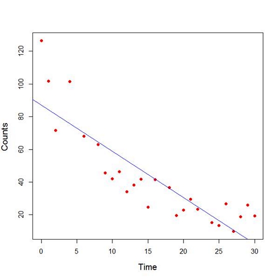
Here the syntax cex.lab = 1.3 produced axis labels of a nice size.
The model looks good, but we can see that the plot has curvature that is not explained well by a linear model. Now we fit a model that is quadratic in time. We create a variable called Time2 which is the square of the variable Time.
Time2 <- Time^2
quadratic.model <-lm(Counts ~ Time + Time2)
Note the syntax involved in fitting a linear model with two or more predictors. We include each predictor and put a plus sign between them.
summary(quadratic.model)
Call:
lm(formula = Counts ~ Time + Time2)
Residuals:
     Min       1Q   Median       3Q     Max
-24.2649 -4.9206 -0.9519   5.5860 18.7728

Coefficients:
             Estimate Std. Error t value Pr(>|t|)
(Intercept) 110.10749   5.48026 20.092 4.38e-16 ***
Time         -7.42253   0.80583 -9.211 3.52e-09 ***
Time2         0.15061   0.02545   5.917 4.95e-06 ***
---
Signif. codes: 0 ‘***’ 0.001 ‘**’ 0.01 ‘*’ 0.05 ‘.’ 0.1 ‘ ’ 1

Residual standard error: 9.754 on 23 degrees of freedom
Multiple R-squared: 0.9014,   Adjusted R-squared: 0.8928
F-statistic: 105.1 on 2 and 23 DF, p-value: 2.701e-12
Our quadratic model is essentially a linear model in two variables, one of which is the square of the other. We see that however good the linear model was, a quadratic model performs even better, explaining an additional 15% of the variance. Now let’s plot the quadratic model by setting up a grid of time values running from 0 to 30 seconds in increments of 0.1s.
timevalues <- seq(0, 30, 0.1)
predictedcounts <- predict(quadratic.model,list(Time=timevalues, Time2=timevalues^2))
plot(Time, Counts, pch=16, xlab = "Time (s)", ylab = "Counts", cex.lab = 1.3, col = "blue")
Now we include the quadratic model to the plot using the lines() command.
lines(timevalues, predictedcounts, col = "darkgreen", lwd = 3)
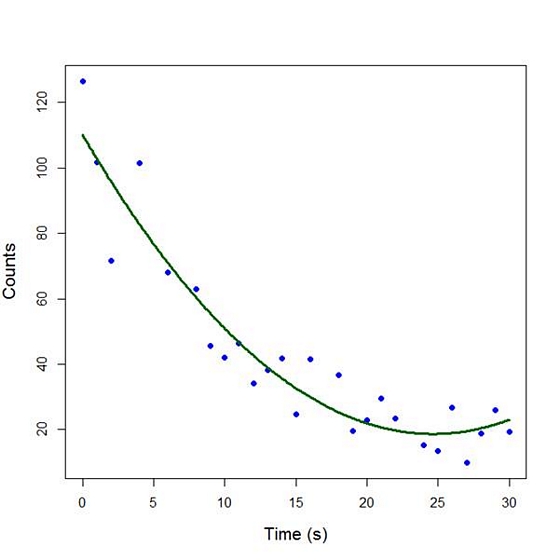
The quadratic model appears to fit the data better than the linear model. We will look again at fitting curved models in our next blog post.
About the Author: David Lillis has taught R to many researchers and statisticians. His company, Sigma Statistics and Research Limited, provides both on-line instruction and face-to-face workshops on R, and coding services in R. David holds a doctorate in applied statistics.
See our full R Tutorial Series and other blog posts regarding R programming.