by Annette Gerritsen, Ph.D.
Cross-tabulation in cohort studies
Assume you have just done a cohort study. How do you actually do the cross-tabulation to calculate the cumulative incidence in both groups?
Best is to always put the outcome variable (disease yes/no) in the columns and the exposure variable in the rows. In other words, put the dependent variable–the one that describes the problem under study–in the columns. And put the independent variable–the factor assumed to cause the problem–in the rows.
Let’s take as example a cohort study used to see whether there is a causal relationship between the use of a certain water source and the incidence of diarrhea among children under five in a village with different water sources. In this case, the variable diarrhea (yes/no) should be in the columns. The variable water source (suspected/other) should be in the rows.
SPSS will put the lowest value of the variable in the first column or row. So in order to get those with diarrhea in the first column you should label ‘diarrhea’ as 1 and ‘no diarrhea’ as 2. The same is true for the exposure variable: label the ‘suspected water source’ as 1 and the ‘other water source’ as 2.
You will then be able to calculate the cumulative incidence (risk of developing the disease) among those with the exposure: a / (a + b) and among those without the exposure: c / (c + d).
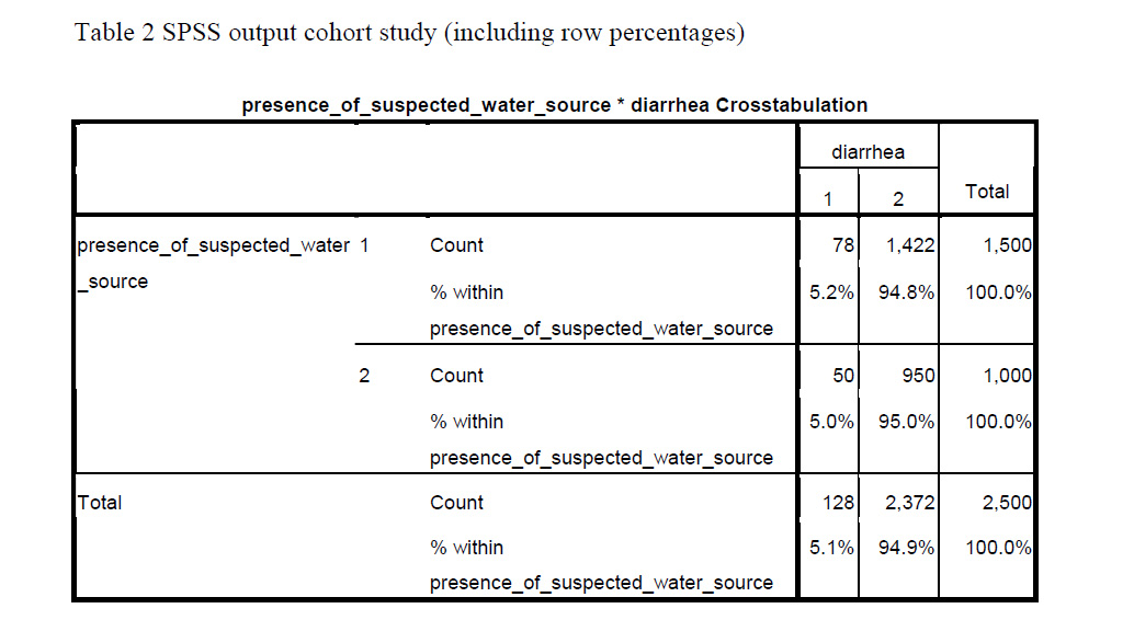
In the case of the diarrhea study (Table 1), you could calculate the cumulative incidence of diarrhea among those exposed to the suspected water source, which would be (78 / 1,500 =) 5.2%.
You can also do this for those exposed to other water sources, which would be (50 / 1,000 =) 5.0%.

SPSS can give you these percentages immediately (in cell ‘a’ and ‘c’ respectively), when you ask to display row percentages in the Cells option (Table 2).

Cross-tabulation in Case-Control Studies
When you have used a case-control design for the diarrhea study, the actual cross-tabulation is quite similar, only “presence of diarrhea yes/no”, is now changed into “cases” and “controls.
Label the cases as 1, and the controls as 2. Be aware that row percentages have no meaning in terms of occurrence of disease in case-control studies. This is because in case-control studies the researcher determines how many patients and how many controls are included.
The ratio between the number of patients and controls (e.g. 2 : 1 or 4 : 1) influences the row percentages. So in a case-control study, the cumulative incidence cannot be calculated.
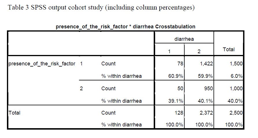
When having conducted a case-control study, you can ask to display column percentages. That gives you the proportion of those exposed to the suspected water source among the cases (in cell ‘a’) and among the controls (in cell ‘b’).
Table 3 gives the SPSS output for the same diarrhea study assuming that it had a case-control design. Using the data provided, (78 / 128 =) 60.9% of the cases were exposed to the suspected water source, while this was (1,422 / 2,372 =) 59.9% of the controls (asked for column percentages).

Another article will be devoted to measures of association: How do you actually compare cumulative incidence rates in cohort studies? And what measure of association can be used in case-control studies?
About the Author: With expertise in epidemiology, biostatistics and quantitative research projects, Annette Gerritsen, Ph.D. provides services to her clients focussing on the methodological soundness of each phase of an epidemiological study to ensure getting valid answers to the proposed research questions. She is the founder of Epi Result.
Have you ever needed to do some major data management in SPSS and ended up with a syntax program that’s pages long? This is the kind you couldn’t even do with the menus, because you’d tear your hair out with frustration because it took you four weeks to create some new variables.
I hope you’ve gotten started using Syntax, which not only gives you a record of how you’ve recoded and created all those new variables and exactly which options you chose in the data analysis you’ve done.
But once you get started, you start to realize that some things feel a little clunky. You have to run the same descriptive analysis on 47 different variables. And while cutting and pasting is a heck of a lot easier than doing that in the menus, you wonder if there isn’t a better way.
There is.
SPSS syntax actually has a number of ways to increase programming efficiency, including macros, do loops, repeats.
I admit I haven’t used this stuff a lot, but I’m increasingly seeing just how useful it can be. I’m much better trained in doing these kinds of things in SAS, so I admit I have been known to just import data into SAS to run manipulations.
But I just came across a great resources on doing sophisticated SPSS Syntax Programming, and it looks like some fabulous bedtime reading. (Seriously).
And the best part is you can download it (or order it, if you’d like a copy to take to bed) from the author’s website, Raynald’s SPSS Tools, itself a great source of info on mastering SPSS.
So once you’ve gotten into the habit of hitting Paste instead of Okay, and gotten a bit used to SPSS syntax, and you’re ready to step your skills up a notch, this looks like a fabulous book.
[Edit]: As per Jon Peck in the comments below, the most recent version is now available at www.ibm.com/developerworks/spssdevcentral under Books and Articles.
Want to learn more? If you’re just getting started with data analysis in SPSS, or would like a thorough refresher, please join us in our online workshop Introduction to Data Analysis in SPSS.
If you’ve ever tried sharing SPSS output with your collaborators, advisor, or statistical consultant, you have surely noticed that the output is often not compatible across different versions of SPSS.
And if you work in a company where everyone is working on the same site license, it’s not a problem. But if you’re collaborating with colleagues at different universities on different upgrade schedules, you might run into some problems.
It’s true that most software programs aren’t back-compatible. You can’t read documents created in newer versions in older versions of software.
But SPSS’s sharing capabilities are more, um, interesting.
The syntax and data files are back and forward-compatible across many versions, at least since v9 or so. (I don’t (more…)
Maybe I’ve noticed it more because I’m getting ready for next week’s SPSS in GLM workshop. Just this week, I’ve had a number of experiences with people’s struggle with SPSS, and GLM in particular.
Number 1: I read this in a technical report by Patrick Burns comparing SPSS to R:
“SPSS is notorious for its attitude of ‘You want to do one of these things. If you don’t understand what the output means, click help and we’ll pop up five lines of mumbo-jumbo that you’re not going to understand either.’ “
And while I still prefer SPSS, I had to laugh because the anonymous person Burns (more…)
I hope you’re getting started using SPSS Syntax by hitting that Paste button when you use the menus.
But there are a few parts of SPSS you can’t do that with. Specifically, there are syntax commands for doing all the variable definitions that you usually fill out in the “Variable View” window. But there are no Paste buttons there, so you have to know how to write the syntax from scratch.
I find the three variable definitions that I use the most are defining Variable Labels, Value Labels and Missing Data codes. The syntax is simple and logical for all three, so I’m going to just give you the basic code, which you can keep on hand and edit as you need.
For a data set with the variables Gender, Smoke, and Exercise, with the following definitions:
Gender: 0=Male, 1=Female
Smoke: 1=Never 2=Sometimes 3=Daily
Exercise: 1=Never 2=Sometimes 3=Daily
For all three variables, 999 = a user-defined missing value
We could use the following code to give descriptive variable labels, encode the value labels, and define the missing data:
VARIABLE LABELS
GENDER ‘Participant Gender’
SMOKE ‘Does Participant ever Smoke Cigarettes?’
EXERCISE ‘How Often Does Participant Exercise for a30 Minute Period?’.
Notice two things:
1. I could put all three Variable labels in the same Variable Label statement
2. There is a period at the end of the statement. This is required.
VALUE LABELS
GENDER 0 ‘Male’ 1 ‘Female
/SMOKE EXERCISE
1 ‘Never’
2 ‘Sometimes’
3 ‘Daily’.
MISSING VALUES
GENDER SMOKE EXERCISE (999).
Since all three variables have the same missing data code, I could include them all in the same statement.
There are, of course syntax rules for all of these commands, but you can easily look them up in the Command Syntax Manual.
Want to learn more? If you’re just getting started with data analysis in SPSS, or would like a thorough refresher, please join us in our online workshop Introduction to Data Analysis in SPSS.
I find SPSS manuals, as a rule, marginally useful. Sure they may tell you which options are available when doing Statistic X, but not what they mean or when to use them.
I still use them, of course, but only when I have no other options.
There is one exception, though, and that is the Command Syntax Reference. This is the manual that explains all the SPSS Syntax commands.
SPSS started as a syntax-only program. I first learned SPSS before Windows existed. I don’t think you could even get it for a PC back then. We had to use the College’s VAX mainframe computer. This was back in the days where you had to go pick up your printouts down the hall in the computing center. But no cards. I’m not THAT old.
Anyway, I think in those days SPSS must have put a lot of resources into really good manual writing. So the Command Syntax Reference, which was the entire manual, rocked. It still does, since for the most part, the syntax doesn’t change that much with new versions.
The great thing about it is now it’s available right in SPSS. When you click on help, instead of Search, choose Command Syntax Reference. It includes every possible option, explains when and how to use it, and what it means. It’s an extremely handy resource, comes free with SPSS, and you don’t have to spend hours searching the internet for an answer.
The only hard part about it is it is organized by the command, and they’re not always intuitive. So if you don’t know that the Univariate GLM menu equivalent syntax command is “UNIANOVA,” you’ll have a hard time using it.
This is another good time to use the Paste button. Just use the menus to create some semblance of the analysis you want to do and hit Paste. You’ll get the basic command, which you can now look up and refine.
Want to learn more? If you’re just getting started with data analysis in SPSS, or would like a thorough refresher, please join us in our online workshop Introduction to Data Analysis in SPSS.


