There’s no mincing words here. Missing values can cause problems for every statistician. That’s true for a lot of reasons, but it can start with simple issues of choices  made when coding missing values in a data set. Here are a few examples.
Example 1: The Null License Plate
Researcher Joseph Tartaro thought it would be funny to get the following California vanity license plate: (more…)
Imputation as an approach to missing data has been around for decades.

You probably learned about mean imputation in methods classes, only to be told to never do it for a variety of very good reasons. Mean imputation, in which each missing value is replaced, or imputed, with the mean of observed values of that variable, is not the only type of imputation, however. (more…)
Missing data are a widespread problem, as most researchers can attest. Whether data are from surveys, experiments, or secondary sources, missing data abounds.
But what’s the impact on the results of statistical analysis? That depends on two things: the mechanism that led the data to be missing and the way in which the data analyst deals with it.
Here are a few common situations:
Subjects in longitudinal studies often start, but drop out before the study is completed. There are many reasons for this: they have moved out of the area (nothing related to the study), died (hopefully not related to the study), no longer see personal benefit to participating, or do not like the effects of the treatment.
Surveys suffer missing data in many ways. When participants refuse to answer the entire survey or parts of it; do not know the answer to, or accidentally skip an item. Some survey researchers even design the study so that some questions are asked of only a subset of participants.
Experimental studies have missing data when a researcher is simply unable to collect an observation. Bad weather conditions may render observation impossible in field experiments. A researcher becomes sick or equipment fails. Data may be missing in any type of study due to accidental or data entry error. A researcher drops a tray of test tubes. A data file becomes corrupt.
Most researchers are very familiar with one (or more) of these situations.
Why Missing Data Matters
Missing data cause problems because most statistical procedures require a value for each variable. When a data set is incomplete, the data analyst has to decide how to deal with it.
The most common decision is to use complete case analysis (also called listwise deletion). This means analyzing only the cases with complete data. Individuals with data missing on any variables are dropped from the analysis.
It has advantages–it is easy to use, is very simple, and is the default in most statistical packages. But it has limitations.
It can substantially lower the sample size, leading to a severe lack of power. This is especially true if there are many variables involved in the analysis, each with data missing for a few cases.
Possibly worse, it can also lead to biased results, depending on why and in which patterns the data are missing.
Missing Data Mechanisms
The types of missing data fit into three classes, which are based on the relationship between the missing data mechanism and the missing and observed values. These badly-named classes are important to understand because the problems caused by missing data and the solutions to these problems are different for the three classes.
Missing Completely at Random
The first is Missing Completely at Random (MCAR). MCAR means that the missing data mechanism is unrelated to the values of any variables, whether missing or observed.
Data that are missing because a researcher dropped the test tubes or survey participants accidentally skipped questions are likely to be MCAR.
If the observed values are essentially a random sample of the full data set, complete case analysis gives the same results as the full data set would have. Unfortunately, most missing data are not MCAR.
Missing Not at Random
At the opposite end of the spectrum is Missing Not at Random. Although you’ll most often see it called this, I prefer the term Non-Ignorable (NI). NI is a name that is not so easy to confuse with the other types, but it also tells you its primary feature. It means that the missing data mechanism is related to the missing values.
And this is something you, the data analyst, can’t ignore without biasing results.
It occurs sometimes when people do not want to reveal something very personal or unpopular about themselves. For example, if individuals with higher incomes are less likely to reveal them on a survey than are individuals with lower incomes, the missing data mechanism for income is non-ignorable. Whether income is missing or observed is related to its value.
But that’s not the only example. When the sickest patients drop out of a longitudinal study testing a drug that’s supposed to make them healthy, that’s non-ignorable.
Or an instrument can’t detect low readings, so gives you an error, also non-ignorable.
Complete case analysis can give highly biased results for NI missing data. If proportionally more low and moderate income individuals are left in the sample because high income people are missing, an estimate of the mean income will be lower than the actual population mean.
Missing at Random
In between these two extremes is Missing at Random (MAR). MAR requires that the cause of the missing data is unrelated to the missing values but may be related to the observed values of other variables.
MAR means that the missing values are related to observed values on other variables. As an example of CD missing data, missing income data may be unrelated to the actual income values but are related to education. Perhaps people with more education are less likely to reveal their income than those with less education.
A key distinction is whether the mechanism is ignorable (i.e., MCAR or MAR) or non-ignorable. There are excellent techniques for handling ignorable missing data. Non-ignorable missing data are more challenging and require a different approach.
First Published 2/24/2014;
Updated 5/11/21 to give more detail.
Mean imputation: So simple. And yet, so dangerous.
Perhaps that’s a bit dramatic, but mean imputation (also called mean substitution) really ought to be a last resort.
It’s a popular solution to missing data, despite its drawbacks. Mainly because it’s easy. It can be really painful to lose a large part of the sample you so carefully collected, only to have little power.
But that doesn’t make it a good solution, and it may not help you find relationships with strong parameter estimates. Even if they exist in the population.
On the other hand, there are many alternatives to mean imputation that provide much more accurate estimates and standard errors, so there really is no excuse to use it.
This post is the first explaining the many reasons not to use mean imputation (and to be fair, its advantages).
First, a definition: mean imputation is the replacement of a missing observation with the mean of the non-missing observations for that variable.
Problem #1: Mean imputation does not preserve the relationships among variables.
True, imputing the mean preserves the mean of the observed data. So if the data are missing completely at random, the estimate of the mean remains unbiased. That’s a good thing.
Plus, by imputing the mean, you are able to keep your sample size up to the full sample size. That’s good too.
This is the original logic involved in mean imputation.
If all you are doing is estimating means (which is rarely the point of research studies), and if the data are missing completely at random, mean imputation will not bias your parameter estimate.
It will still bias your standard error, but I will get to that in another post.
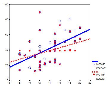
Since most research studies are interested in the relationship among variables, mean imputation is not a good solution. The following graph illustrates this well:

This graph illustrates hypothetical data between X=years of education and Y=annual income in thousands with n=50. The blue circles are the original data, and the solid blue line indicates the best fit regression line for the full data set. The correlation between X and Y is r = .53.
I then randomly deleted 12 observations of income (Y) and substituted the mean. The red dots are the mean-imputed data.
Blue circles with red dots inside them represent non-missing data. Empty Blue circles represent the missing data. If you look across the graph at Y = 39, you will see a row of red dots without blue circles. These represent the imputed values.
The dotted red line is the new best fit regression line with the imputed data. As you can see, it is less steep than the original line. Adding in those red dots pulled it down.
The new correlation is r = .39. That’s a lot smaller that .53.
The real relationship is quite underestimated.
Of course, in a real data set, you wouldn’t notice so easily the bias you’re introducing. This is one of those situations where in trying to solve the lowered sample size, you create a bigger problem.
One note: if X were missing instead of Y, mean substitution would artificially inflate the correlation.
In other words, you’ll think there is a stronger relationship than there really is. That’s not good either. It’s not reproducible and you don’t want to be overstating real results.
This solution that is so good at preserving unbiased estimates for the mean isn’t so good for unbiased estimates of relationships.
Problem #2: Mean Imputation Leads to An Underestimate of Standard Errors
A second reason is applies to any type of single imputation. Any statistic that uses the imputed data will have a standard error that’s too low.
In other words, yes, you get the same mean from mean-imputed data that you would have gotten without the imputations. And yes, there are circumstances where that mean is unbiased. Even so, the standard error of that mean will be too small.
Because the imputations are themselves estimates, there is some error associated with them. But your statistical software doesn’t know that. It treats it as real data.
Ultimately, because your standard errors are too low, so are your p-values. Now you’re making Type I errors without realizing it.
That’s not good.
A better approach? There are two: Multiple Imputation or Full Information Maximum Likelihood.
A data set can contain indicator (dummy) variables, categorical variables and/or both. Initially, it all depends upon how the data is coded as to which variable type it is.
For example, a categorical variable like marital status could be coded in the data set as a single variable with 5 values: (more…)
In the last post, we examined how to use the same sample when running a set of regression models with different predictors.
Adding a predictor with missing data causes cases that had been included in previous models to be dropped from the new model.
Using different samples in different models can lead to very different conclusions when interpreting results.
Let’s look at how to investigate the effect of the missing data on the regression models in Stata.
The coefficient for the variable “frequent religious attendance” was negative 58 in model 3 and then rose to a positive 6 in model 4 when income was included. Results (more…)
 made when coding missing values in a data set. Here are a few examples.

