 Sometimes when you’re learning a new stat software package, the most frustrating part is not knowing how to do very basic things. This is especially frustrating if you already know how to do them in some other software.
Let’s look at some basic but very useful commands that are available in R.
We will use the following data set of tourists from different nations, their gender and numbers of children. Copy and paste the following array into R.
A <- structure(list(NATION = structure(c(3L, 3L, 3L, 1L, 3L, 2L, 3L,
1L, 3L, 3L, 1L, 2L, 2L, 3L, 3L, 3L, 2L), .Label = c("CHINA",
"GERMANY", "FRANCE"), class = "factor"), GENDER = structure(c(1L,
2L, 2L, 1L, 2L, 1L, 2L, 1L, 2L, 2L, 1L, 1L, 1L, 1L, 2L, 1L, 1L
), .Label = c("F", "M"), class = "factor"), CHILDREN = c(1L,
3L, 2L, 2L, 3L, 1L, 0L, 1L, 0L, 1L, 2L, 2L, 1L, 1L, 1L, 0L, 2L
)), .Names = c("NATION", "GENDER", "CHILDREN"), row.names = 2:18, class = "data.frame")
Want to check that R read the variables correctly? We can look at the first 3 rows using the head() command, as follows:
head(A, 3)
  NATION   GENDER   CHILDREN
2 FRANCE      F        1
3 FRANCE      M        3
4 FRANCE      M        2
Now we look at the last 4 rows using the tail() command:
tail(A, 4)
    NATION   GENDER  CHILDREN
15  FRANCE      F        1
16  FRANCE      M        1
17  FRANCE      F        0
18 GERMANY      F        2
Now we find the number of rows and number of columns using nrow() and ncol().
nrow(A)
[1] 17

ncol(A)
[1] 3
So we have 17 rows (cases) and three columns (variables). These functions look very basic, but they turn out to be very useful if you want to write R-based software to analyse data sets of different dimensions.
Now let’s attach A and check for the existence of particular data.
attach(A)
As you may know, attaching a data object makes it possible to refer to any variable by name, without having to specify the data object which contains that variable.
Does the USA appear in the NATION variable? We use the any() command and put USA inside quotation marks.
any(NATION == "USA")
[1] FALSE
Clearly, we do not have any data pertaining to the USA.
What are the values of the variable NATION?
levels(NATION)
[1] "CHINA"   "GERMANY" "FRANCE"
How many non-missing observations do we have in the variable NATION?
length(NATION)
[1] 17
OK, but how many different values of NATION do we have?
length(levels(NATION))
[1] 3
We have three different values.
Do we have tourists with more than three children? We use the any() command to find out.
any(CHILDREN > 3)
[1] FALSE
None of the tourists in this data set have more than three children.
Do we have any missing data in this data set?
In R, missing data is indicated in the data set with NA.
any(is.na(A))
[1] FALSE
We have no missing data here.
Which observations involve FRANCE? We use the which() command to identify the relevant indices, counting column-wise.
which(A == "FRANCE")
[1]  1  2  3  5  7  9 10 14 15 16
How many observations involve FRANCE? We wrap the above syntax inside the length() command to perform this calculation.
length(which(A == "FRANCE"))
[1] 10
We have a total of ten such observations.
That wasn’t so hard! In our next post we will look at further analytic techniques in R.
About the Author: David Lillis has taught R to many researchers and statisticians. His company, Sigma Statistics and Research Limited, provides both on-line instruction and face-to-face workshops on R, and coding services in R. David holds a doctorate in applied statistics.
See our full R Tutorial Series and other blog posts regarding R programming.

In my last article, Hierarchical Regression in Stata: An Easy Method to Compare Model Results, I presented the following table which examined the impact several predictors have on one’ mental health.
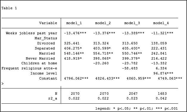
At the bottom of the table is the number of observations (N) contained within each sample.
The sample sizes are quite large. Does it really matter that they are different? The answer is absolutely yes.
Fortunately in Stata it is not a difficult process to use the same sample for all four models shown above.
Some background info:
As I have mentioned previously, Stata stores results in temp files. You don’t have to do anything to cause Stata to store these results, but if you’d like to use them, you need to know what they’re called.
To see what is stored after an estimation command, use the following code:
ereturn list
After a summary command:
return list
One of the stored results after an estimation command is the function e(sample). e(sample) returns a one column matrix. If an observation is used in the estimation command it will have a value of 1 in this matrix. If it is not used it will have a value of 0.
Remember that the “stored” results are in temp files. They will disappear the next time you run another estimation command.
The Steps
So how do I use the same sample for all my models? Follow these steps.
Using the regression example on mental health I determine which model has the fewest observations. In this case it was model four.
I rerun the model:
regress MCS weeks_unemployed i.marital_status kids_in_house religious_attend income
Next I use the generate command to create a new variable whose value is 1 if the observation was in the model and 0 if the observation was not. I will name the new variable “in_model_4”.
gen in_model_4 = e(sample)
Now I will re-run my four regressions and include only the observations that were used in model 4. I will store the models using different names so that I can compare them to the original models.
My commands to run the models are:
regress MCS weeks_unemployed i.marital_status if in_model_4==1
estimates store model_1a
regress MCS weeks_unemployed i.marital_status kids_in_house if in_model_4==1
estimates store model_2a
regress MCS weeks_unemployed i.marital_status kids_in_house religious_attend if in_model_4==1
estimates store model_3a
regress MCS weeks_unemployed i.marital_status kids_in_house religious_attend income if in_model_4==1
estimates store model_4a
Note: I could use the code if in_model_4 instead of if in_model_4==1. Stata interprets dummy variables as 0 = false, 1 = true.
Here are the results comparing the original models (eg. Model_1) versus the models using the same sample (eg. Model_1a):
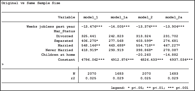
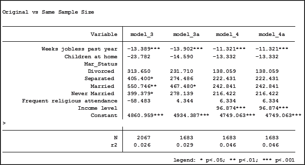
Comparing the original models 3 and 4 one would have assumed that the predictor variable “Income level” significantly impacted the coefficient of “Frequent religious attendance”. Its coefficient changed from -58.48 in model 3 to 6.33 in model 4.
That would have been the wrong assumption. That change is coefficient was not so much about any effect of the variable itself, but about the way it causes the sample to change via listwise deletion. Using the same sample, the change in the coefficient between the two models is very small, moving from 4 to 6.
Jeff Meyer is a statistical consultant with The Analysis Factor, a stats mentor for Statistically Speaking membership, and a workshop instructor. Read more about Jeff here.
Have you ever worked with a data set that had so many observations and/or variables that you couldn’t see the forest for the trees? You would like to extract some simple information but you can’t quite figure out how to do it.
Get to know Stata’s collapse command–it’s your new friend. Collapse allows you to convert your current data set to a much smaller data set of means, medians, maximums, minimums, count or percentiles (your choice of which percentile).
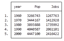
Let’s take a look at an example. I’m currently looking at a longitudinal data set filled with economic data on all 67 counties in Alabama. The time frame is in decades, from 1960 to 2000. Five time periods by 67 counties give me a total of 335 observations.
What if I wanted to see some trend information, such as the total population and jobs per decade for all of Alabama? I just want a simple table to see my results as well as a graph. I want results that I can copy and paste into a Word document.
Here’s my code:
preserve

collapse (sum) Pop Jobs, by(year)

graph twoway (line Pop year) (line Jobs year), ylabel(, angle(horizontal))

list
And here is my output:
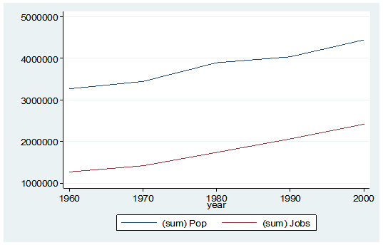
By starting my code with the preserve command it brings my data set back to its original state after providing me with the results I want.
What if I want to look at variables that are in percentages, such as percent of college graduates, mobility and labor force participation rate (lfp)? In this case I don’t want to sum the values because they are in percent.
Calculating the mean would give equal weighting to all counties regardless of size.
Fortunately Stata gives you a very simple way to weight your data based on frequency. You have to determine which variable to use. In this situation I will use the population variable.
Here’s my coding and results:
Preserve

collapse (mean) lfp College Mobil [fw=Pop], by(year)

graph twoway (line lfp year) (line College year) (line Mobil year), ylabel(, angle(horizontal))

list
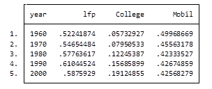
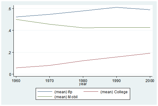
It’s as easy as that. This is one of the five tips and tricks I’ll be discussing during the free Stata webinar on Wednesday, July 29th.
Jeff Meyer is a statistical consultant with The Analysis Factor, a stats mentor for Statistically Speaking membership, and a workshop instructor. Read more about Jeff here.
Stata allows you to describe, graph, manipulate and analyze your data in countless ways. But at times (many times) it can be very frustrating trying to create even the simplest results. Join us and learn how to reduce your future frustrations.
This one hour demonstration is for new and intermediate users of Stata. If you’re a beginner, the drop down commands can be extremely daunting.
If you’re an intermediate user and not constantly using Stata, it’s impossible to remember which commands generate the results you are looking to create.
 This webinar, by guest presenter Jeff Meyer, will give you five actionable tips (and examples you can re-use) that will make your next analysis in Stata much simpler.
We’ll explore:
- Save time with a do-file to create the table you want exactly as you want.
- A few methods (some easier than others) to create dummy variables out of a categorical variable with several categories
- At least three ways to insert a table into a document
- Quickly alter the looks of your graphs through the use of macros
- How to aggregate data to the group level based on a number of parameters
Date: Wednesday, July 29, 2015
Time: 4pm EDT (New York time)
Cost: Free
***Note: This webinar has already taken place. Sign up below to get access to the video recording of the webinar.
Our next free webinar is titled: “Random Intercept and Random Slope Models” and is coming up in August
Jeff Meyer is a statistical consultant with The Analysis Factor, a stats mentor for Statistically Speaking membership, and a workshop instructor. Read more about Jeff here.