If you’re like most researchers, your statistical training focused on Regression or ANOVA, but not both. It all depends on whether your field focuses more on experimental data (Biology, Psychology) or observed data (Sociology, Economics). Maybe one class covered a bit of the other, but most people are comfortable in one, but not the other.
This, in my opinion, is a shame. (Okay, I was going to say tragedy, but let’s be real. Tsunami that kills thousands=tragedy. Different scale here).
First of all, the distinction between ANOVA and linear regression is arbitrary. They’re really the same model with different outfits on.
Second, regardless of which one you normally use, you’re going to occasionally have to use the other kind of predictor variables–categorical or continuous. And we can come up with nice names for these models–a regression with dummy variables or an Analysis of Covariance.
But real understanding of the relationships among variables comes only when you dispense of the names and can focus on analyzing and interpreting the model using the kinds of variables you have.
There are other examples, but today I’m going to focus on an ANOVA model with a continuous covariate.
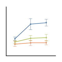
A common model is one in which one predictor is categorical (we’ll use 4 categories) and the other is continuous. Here is an example of a scatterplot of just such a model:

There are four groups, each of which received a different training. The continuous moderator is Age, and the outcome is OverallPost, which is the post-training test score to see how well they learned the material in each training program.
As you can see, the effect of the training program is moderated by age. Another way to say that is there is a significant interaction between Age and Training Group. The effect of the training is depending on the trainee’s age.
One way to interpret this significant interaction is to compare the slopes of the four lines, which is easily done with any regression coefficient table. (Okay, not always easily done, but easily found in…)
But this doesn’t make very much sense when Age is really a moderator–a predictor we want to control for, and see how it affects the relationship between the independent (IV) and dependent variables (DV), but not really the IV we’re interested in.
A better way to do it in this situation is to compare the means among groups at a low value of Age, say 20, and again at a high value of Age, say 50. You can get p-values, adjusted for multiple comparisons, using either SAS or SPSS GLM.
SAS Proc GLM uses the LSMeans statement and SPSS GLM uses EMMeans. They do the same thing–calculate the mean of Y for each group, at a specific value of the covariate.
If you use the menus in SPSS, you can only get those EMMeans at the Covariate’s mean, which in this example is about 25, where the vertical black line is. This isn’t very useful for our purposes. But we can change the value of the covariate at which to compare the means using syntax.
So it would tell us that at a young age of say 20, the three treatment groups (green, tan, and purple lines) all have means higher than the control (blue). Young people learned more in all three treatment groups.
But at an older age, say 50, the means of the purple and tan groups were not significantly different from the control group’s (blue), and the green (EIQ group) did worse!
In SPSS GLM, the syntax would be:
UNIANOVA OverallPost BY group WITH NEWAGE
/METHOD=SSTYPE(3)
/INTERCEPT=INCLUDE
/EMMEANS=TABLES(group) WITH(NEWAGE=MEAN) COMPARE ADJ(SIDAK)
/EMMEANS=TABLES(group) WITH(NEWAGE=45) COMPARE ADJ(SIDAK)
/EMMEANS=TABLES(group) WITH(NEWAGE=20) COMPARE ADJ(SIDAK)
/PRINT=PARAMETER
/CRITERIA=ALPHA(.05)
/DESIGN=NEWAGE group NEWAGE*group.