Of all the concepts I see researchers struggle with as they start to learn high-level statistics, the one that seems to most often elicit the blank stare of incomprehension is the Covariance Matrix, and its friend, the Covariance Structure.
And since understanding them is fundamental to a number of statistical analyses, particularly Mixed Models and Structural Equation Modeling, it’s an incomprehension you can’t afford.
So I’m going to explain what they are and how they’re not so different from what you’re used to. I hope you’ll see that once you get to know them, they aren’t so scary after all.
What is a Covariance Matrix?
There are two concepts inherent in a covariance matrix–covariance and matrix. Either one can throw you off.
Let’s start with matrix. If you never took linear algebra, the idea of matrices can be frightening. (And if you still are in school, I highly recommend you take it. Highly). And there are a lot of very complicated, mathematical things you can do with matrices.
But you, a researcher and data analyst, don’t need to be able to do all those complicated processes to your matrices. You do need to understand what a matrix is, be able to follow the notation, and understand a few simple matrix processes, like multiplication of a matrix by a constant.
The thing to keep in mind when it all gets overwhelming is a matrix is just a table. That’s it.
A Covariance Matrix, like many matrices used in statistics, is symmetric. That means that the table has the same headings across the top as it does along the side.
Start with a Correlation Matrix
The simplest example, and a cousin of a covariance matrix, is a correlation matrix. It’s just a table in which each variable is listed in both the column headings and row headings, and each cell of the table (i.e. matrix) is the correlation between the variables that make up the column and row headings. Here is a simple example from a data set on 62 species of mammal:
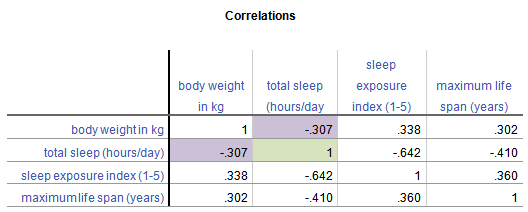
From this table, you can see that the correlation between Weight in kg and Hours of Sleep, highlighted in purple, is -.307. Smaller mammals tend to sleep more.
You’ll notice that this is the same above and below the diagonal. The correlation of Hours of Sleep with Weight in kg is the same as the correlation between Weight in kg and Hours of Sleep.
Likewise, all correlations on the diagonal equal 1, because they’re the correlation of each variable with itself.
If this table were written as a matrix, you’d only see the numbers, without the column headings.
Now, the Covariance Matrix
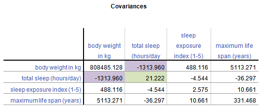
A Covariance Matrix is very similar. There are really two differences between it and the Correlation Matrix. It has this form:

First, we have substituted the correlation values with covariances.
Covariance is just an unstandardized version of correlation. To compute any correlation, we divide the covariance by the standard deviation of both variables to remove units of measurement. So a covariance is just a correlation measured in the units of the original variables.
Covariance, unlike correlation, is not constrained to being between -1 and 1. But the covariance’s sign will always be the same as the corresponding correlation’s. And a covariance=0 has the exact same meaning as a correlation=0: no linear relationship.
Because covariance is in the original units of the variables, variables on scales with bigger numbers and with wider distributions will necessarily have bigger covariances. So for example, Life Span has similar correlations to Weight and Exposure while sleeping, both around .3.
But values of Weight vary a lot (this data set contains both Elephants and Shrews), whereas Exposure is an index variable that ranges from only 1 to 5. So Life Span’s covariance with Weight (5113.27) is much larger than than with Exposure (10.66).
Second, the diagonal cells of the matrix contain the variances of each variable. A covariance of a variable with itself is simply the variance. So you have a context for interpreting these covariance values.
Once again, a covariance matrix is just the table without the row and column headings.
What about Covariance Structures?
Covariance Structures are just patterns in covariance matrices. Some of these patterns occur often enough in some statistical procedures that they have names.
You may have heard of some of these names–Compound Symmetry, Variance Components, Unstructured, for example. They sound strange because they’re often thrown about without any explanation.
But they’re just descriptions of patterns.
For example, the Compound Symmetry structure just means that all the variances are equal to each other and all the covariances are equal to each other. That’s it.
It wouldn’t make sense with our animal data set because each variable is measured on a different scale. But if all four variables were measured on the same scale, or better yet, if they were all the same variable measured under four experimental conditions, it’s a very plausible pattern.
Variance Components just means that each variance is different, and all covariances=0. So if all four variables were completely independent of each other and measured on different scales, that would be a reasonable pattern.
Unstructured just means there is no pattern at all. Each variance and each covariance is completely different and has no relation to the others.
There are many, many covariance structures. And each one makes sense in certain statistical situations. Until you’ve encountered those situations, they look crazy. But each one is just describing a pattern that makes sense in some situations.


 This is where statistical analysis starts to feel really hard. You’re combining two difficult issues into one.