We often talk about nested factors in mixed models — students nested in classes, observations nested within subject.
But in all but the simplest designs, it’s not that straightforward. (more…)
We often talk about nested factors in mixed models — students nested in classes, observations nested within subject.
But in all but the simplest designs, it’s not that straightforward. (more…)
Here’s a common situation.
Your grant application or committee requires sample size estimates. It’s not the calculations that are hard (though they can be), it’s getting the information to fill into the calculations.
Every article you read on it says you need to either use pilot data or another similar study as a basis for the values to enter into the software.
You have neither.
No similar studies have ever used the scale you’re using for the dependent variable.
And while you’d love to run a pilot study, it’s just not possible. There are too many practical constraints — time, money, distance, ethics.
What do you do?
I recently gave a free webinar on Principal Component Analysis. We had almost 300 researchers attend and didn’t get through all the questions. This is part of a series of answers to those questions.
If you missed it, you can get the webinar recording here.
Answer:
Great question. Of course, the answer depends on your situation.
When you retain only one factor in a solution, then rotation is irrelevant. In fact, most software won’t even print out rotated coefficients and they’re pretty meaningless in that situation.
But if you retain two or more factors, you need to rotate.
Unrotated factors are pretty difficult to interpret in that situation. (more…)
I recently gave a free webinar on Principal Component Analysis. We had almost 300 researchers attend and didn’t get through all the questions. This is part of a series of answers to those questions.
If you missed it, you can get the webinar recording here.
Answer: Yes and no.
Principal Component Analysis specifically could be used with a training and test data set, but it doesn’t make as much sense as doing so for Factor Analysis.
That’s because PCA is really just about creating an index variable from a set of correlated predictors.
Factor Analysis is an actual model that is measuring a latent variable. Any time you’re creating some sort of scale to measure an underlying construct, you want to use Factor Analysis.
Factor Analysis is definitely best done with a training and test data set.
In fact, ideally, you’d run multiple rounds of training and test data sets, in which the variables included on your scale are updated after each test. (more…)
I recently gave a free webinar on Principal Component Analysis. We had almost 300 researchers attend and didn’t get through all the questions. This is part of a series of answers to those questions.
If you missed it, you can get the webinar recording here.
In fact, there were a few related but separate questions about using and interpreting the resulting component scores, so I’ll answer them together here.
Answer:
So yes, the point of PCA is to reduce variables — create an index score variable that is an optimally weighted combination of a group of correlated variables.
And yes, you can use this index variable as either a predictor or response variable.
It is often used as a solution for multicollinearity among predictor variables in a regression model. Rather than include multiple correlated predictors, none of which is significant, if you can combine them using PCA, then use that.
It’s also used as a solution to avoid inflated familywise Type I error caused by running the same analysis on multiple correlated outcome variables. Combine the correlated outcomes using PCA, then use that as the single outcome variable. (This is, incidentally, what MANOVA does).
In both cases, you can no longer interpret the individual variables.
You may want to, but you can’t. (more…)
One of the many confusing issues in statistics is the confusion between Principal Component Analysis (PCA) and Factor Analysis (FA).
They are very similar in many ways, so it’s not hard to see why they’re so often confused. They appear to be different varieties of the same analysis rather than two different methods. Yet there is a fundamental difference between them that has huge effects on how to use them.
(Like donkeys and zebras. They seem to differ only by color until you try to ride one).
Both are data reduction techniques—they allow you to capture the variance in variables in a smaller set.
Both are usually run in stat software using the same procedure, and the output looks pretty much the same.
The steps you take to run them are the same—extraction, interpretation, rotation, choosing the number of factors or components.
Despite all these similarities, there is a fundamental difference between them: PCA is a linear combination of variables; Factor Analysis is a measurement model of a latent variable.
PCA’s approach to data reduction is to create one or more index variables from a larger set of measured variables. It does this using a linear combination (basically a weighted average) of a set of variables. The created index variables are called components.
The whole point of the PCA is to figure out how to do this in an optimal way: the optimal number of components, the optimal choice of measured variables for each component, and the optimal weights.
The picture below shows what a PCA is doing to combine 4 measured (Y) variables into a single component, C. You can see from the direction of the arrows that the Y variables contribute to the component variable. The weights allow this combination to emphasize some Y variables more than others.
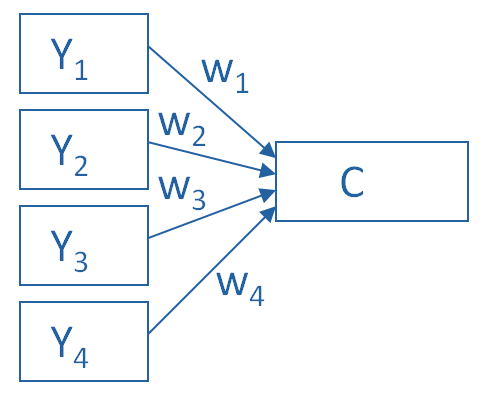
This model can be set up as a simple equation:
C = w1(Y1) + w2(Y2) + w3(Y3) + w4(Y4)
A Factor Analysis approaches data reduction in a fundamentally different way. It is a model of the measurement of a latent variable. This latent variable cannot be directly measured with a single variable (think: intelligence, social anxiety, soil health). Instead, it is seen through the relationships it causes in a set of Y variables.
For example, we may not be able to directly measure social anxiety. But we can measure whether social anxiety is high or low with a set of variables like “I am uncomfortable in large groups” and “I get nervous talking with strangers.” People with high social anxiety will give similar high responses to these variables because of their high social anxiety. Likewise, people with low social anxiety will give similar low responses to these variables because of their low social anxiety.
The measurement model for a simple, one-factor model looks like the diagram below. It’s counter intuitive, but F, the latent Factor, is causing the responses on the four measured Y variables. So the arrows go in the opposite direction from PCA. Just like in PCA, the relationships between F and each Y are weighted, and the factor analysis is figuring out the optimal weights.
In this model we have is a set of error terms. These are designated by the u’s. This is the variance in each Y that is unexplained by the factor.
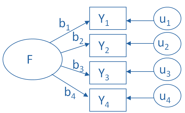
You can literally interpret this model as a set of regression equations:
Y1 = b1*F + u1
Y2 = b2*F + u2
Y3 = b3*F + u3
Y4 = b4*F + u4
As you can probably guess, this fundamental difference has many, many implications. These are important to understand if you’re ever deciding which approach to use in a specific situation.