Regression Models: How do you know you need a polynomial term?

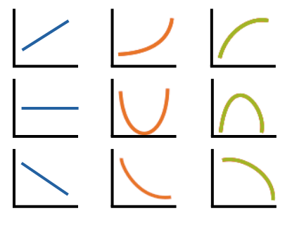
You might be surprised to hear that not only can linear regression fit lines between a response variable Y and one or more predictor variables, X, it can fit curves too. There are many ways to do this, but the simplest is by adding a polynomial term.

So what is a polynomial term and how do you know you need one?

The linear parameters in a regression model

A linear regression model has a few key parameters. These include the intercept coefficient, the slope coefficient, and the residual variance.

That intercept defines the height of the regression line. It does so by measuring the height of the line at one specific point: when all X = 0.

The slope defines how much Y differs, on average, for each one unit difference in X. In other words, it measures the constant relationship between X and Y. Yes, there can be multiple Xs and each one has its own slope.

A polynomial term–a quadratic (squared) or cubic (cubed) term turns a linear regression model into a curve.

Polynomial Regression

When you add a quadratic term, X², to the model, you turn a line into a simple curve, a curve with one “hump”–  a U or inverted U shape.  The curve does not need to contain both sides of the U.  It can contain just part of it.

If you also add a cubic term, X³, your curve now has two humps–one facing upward and the other down.  The curve goes down, back up, then back down again (or vice-versa).

But how do you know if you need one or both of these–when a line isn’t the best model?

There are three main situations that indicate a linear relationship may not be a good model.

1. Theory

Most important is the theoretical one.  There are some relationships that a researcher will hypothesize is curvilinear.  Clearly, if this is the case, include a polynomial term.

You may not keep it.

2. Graph it!

The second chance is during visual inspection of your variables.  This is one of those reasons for always doing univariate and bivariate inspections of your data before you begin your regression analyses.  (You always do this, right?)

A simple scatter plot can reveal a curvilinear relationship.

3. Inspection of residuals.

If you try to fit a linear model to curved data, a scatter plot of residuals (Y axis) on the predictor (X axis) will have patches of many positive residuals in the middle, but patches of negative residuals at either end (or vice versa).  This is a good sign that a linear model is not appropriate, and a polynomial may do better.

Interpreting Linear Regression Coefficients: A Walk Through Output

Learn the approach for understanding coefficients in that regression as we walk through output of a model that includes numerical and categorical predictors and an interaction.

Take Me to The Video!