The linear model normality assumption, along with constant variance assumption, is quite robust to departures. That means that even if the 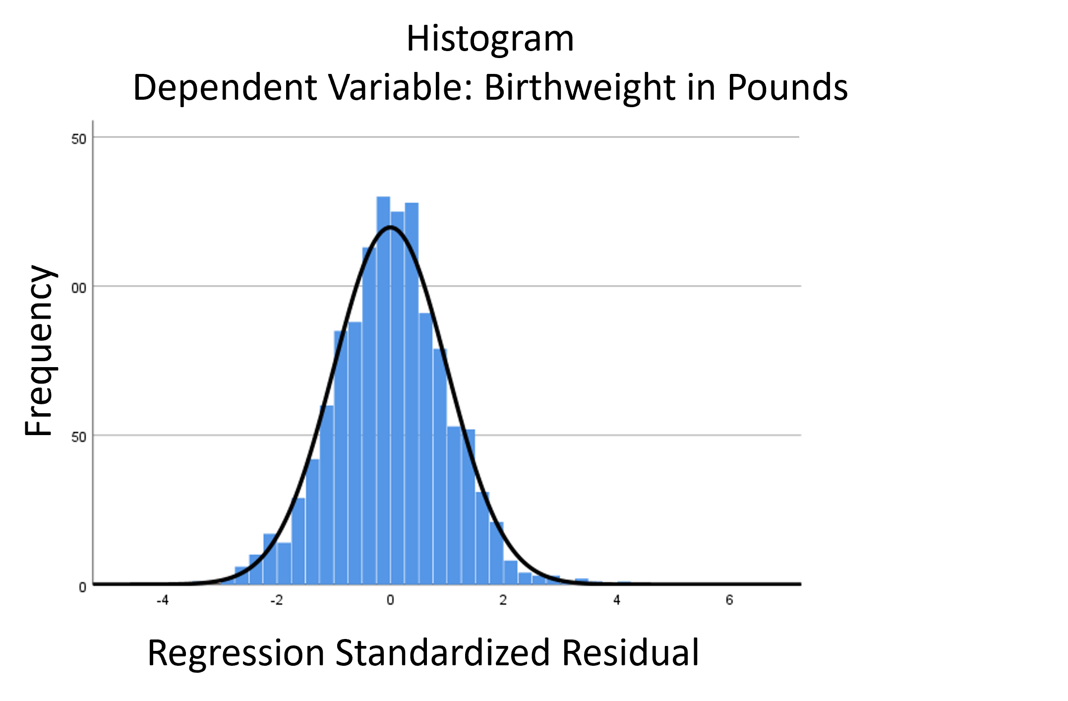 assumptions aren’t met perfectly, the resulting p-values and confidence intervals will still be reasonable estimates.
This is great because it gives you a bit of leeway to run linear models, which are intuitive and (relatively) straightforward. This is true for both linear regression and ANOVA.
You do need to check the assumptions anyway, though. You can’t just claim robustness and not check. Why? Because some departures are so far off that the p-values and confidence intervals become inaccurate. And in many cases there are remedial measures you can take to turn non-normal residuals into normal ones.
But sometimes you can’t.
Sometimes it’s because the dependent variable just isn’t appropriate for a linear model. The dependent variable, Y, doesn’t have to be normally distributed for the errors to be normal (since Y is affected by the X’s).
But the distribution of the errors is related to the distribution of Y. So Y does have to be continuous, unbounded, and measured on an interval or ratio scale.
If those conditions are met, you might have errors that are normally distributed. This is the situation where you can proceed with a linear model and then check the assumptions using the model residuals.
 If you go through the Steps to Statistical Modeling, Step 3 is: Choose the variables for answering your research questions and determine their level of measurement. Part of the reason for doing this is to save yourself from running a model on a DV that just isn’t appropriate and will never meet assumptions.
Because if those conditions are not met, you’re pretty much guaranteed that assumptions won’t be met.
There is, however, some nuance
As with everything in applying statistics, there is some nuance to all three conditions, so let’s address that first.
Continuous
Technically, you need a continuous DV. However, there are some discrete variables with SO many values that they start to appear continuous. And on the scale at which they’re measured, it’s impossible to say.
Take as an example the number of employees in a Fortune 1000 company. These are big companies. Technically, number of employees is discrete. You can’t have 15,401.2 employees.
However, if you look at the distribution across 1000 companies, there are so many different values the variable approaches continuous.
Unbounded
 Technically, a normal distribution runs from -∞ to ∞.
And when a variable has boundaries on its values, the limitations on the values of Y limit the values of the errors.
But again, that’s all theoretical. Practically, almost all values in a normal distribution are within three standard deviations of the mean. So even if there are theoretical boundaries (like an age that can’t be below 0), it may not affect the assumptions much.
Measured on an interval or ratio scale
What this really comes down to is that the variable has to be truly numerical. Not ordered categories that we assigned numbers to. A one point difference between each value has to mean the same thing everywhere along the scale.
This tends to be an issue with ordinal variables, when we assign numbers to what are really ordered categories.
Six types of dependent variables that tend to fail these conditions:
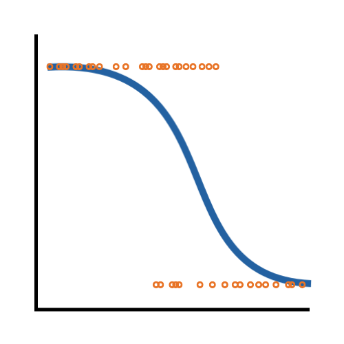
1. Categorical variables come in a few forms: binary (two categories, like yes/no); unordered multicategory (like married, never married, divorced, widowed); and ordered multicategory (listed below).
2. Ordinal variables can be ranks, ordered categories, or Likert scale items.

3. Discrete counts, bounded at 0, which is often the most common value. Especially if the mean is below 10.
4. Zero Inflated, where even if the rest of the distribution looks normal, there is a huge spike in the distribution at 0.
5. Censored or truncated, including time to event variables.
6. Proportions, which are bounded at 0 and 1, or percentages, which are bounded at 0 and 100.
If you have one of these, Stop. Do not pass Go. Do not run a linear model. You will not meet the linear model normality assumption.
Hopefully you noticed this at Step 3, and this helped you plan the statistical analysis. Not when you’re checking assumptions, which is Step 11.
But luckily, there are other types of regression procedures available for all of these variables.
Originally published: 9/17/2009
Last Updated: 2/18/2025
Leave a Reply