| A Note From Karen
 Have you ever noticed that some of the most useful statistics are completely no-intuitive when you first encounter them? Have you ever noticed that some of the most useful statistics are completely no-intuitive when you first encounter them?
Sometimes it takes a little bit of breaking the statistic apart to see what its doing in a particular context.
This month’s newsletter is about one of those, Intraclass Correlation (ICC). It’s a bit of a mouthfeel to say and a little strange at first, but very useful within a few statistical concepts, including mixed models.
I hope you find it useful.
In the meantime, we’ve got a few things in the works.
One is some great workshops for the fall, including two brand new ones by two different guest instructors. I will reveal more once those plans are firmed up.
Over the next few weeks, we hope to unveil (as it were) on demand versions of some of our favorite workshops. We have added to our team a new techy user experience person who is currently putting them together in a way that makes it easy to navigate. Again, we’ll let you know once that is available.
And, if you’re currently, or just contemplating, working with me one-on-one, I will be away (and without internet) for the middle two weeks of August. So please get in touch in the next few weeks so that we can get you on the calendar.
Happy analyzing!
Karen
Feature Article: The Intraclass Correlation Coefficient in Mixed Models
The ICC, or Intraclass Correlation Coefficient, can be very useful in many statistical situations, but especially so in Linear Mixed Models.
Linear Mixed Models are used when there is some sort of clustering in the data.
Two common examples of clustered data include:
- individuals were sampled within sites (hospitals, companies, community centers, schools, etc.). The site is the cluster.
- repeated measures or longitudinal data where multiple observations are collected from the same individual. The individual is the cluster in which multiple observations are grouped.
 Observations from the same cluster are usually more similar to each other than observations from different clusters. If they are, you can’t use statistical methods on these data to that assume independence, because estimates of variance, and therefore p-values, will be incorrect. Observations from the same cluster are usually more similar to each other than observations from different clusters. If they are, you can’t use statistical methods on these data to that assume independence, because estimates of variance, and therefore p-values, will be incorrect.
Mixed models not only account for the correlations among observations in the same cluster, they give you an estimate of that correlation.
At the right is the equation of a very simple linear mixed model. This has a single fixed independent variable, X, and a single random effect u. For simplicity, I’m going to assume that X is centered on it’s mean. This is also known as a random intercept model.
The subscripts i and j on the Y indicate that each observation j is nested within cluster i.
The u represents the random intercept for each cluster. It’s really a residual term that measures the distance from each subject’s intercept around the overall intercept β0. Rather than calculate an estimate for every one of those distances, the model is able to just estimate a single variance σ0.
That variance parameter estimate is the between-cluster variance. The variance of the residuals is the within-cluster variance. Their sum is the total variance in Y that is not explained by X.
 If there is no real correlation among observations within a cluster, the cluster means won’t differ. It’s only when some clusters have generally high values and others have relatively low values that the values within a cluster are correlated. If there is no real correlation among observations within a cluster, the cluster means won’t differ. It’s only when some clusters have generally high values and others have relatively low values that the values within a cluster are correlated.
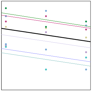
In the graph on the right, each cluster has its own trajectory of a different color. The thick black line represents the overall trajectory, averaged across all clusters.
Some clusters, like the magenta one, have all three values above the overall (black) mean. Those values will be correlated, because they’re all relatively high. Simultaneously, those three points have a high mean.
Likewise, the turquoise cluster has all three values below the overall (black) mean. Again, those values will be correlated, because they’re all relatively low. And the turquoise mean is quite low.
And so it goes. When some clusters have generally high values and others have generally low, (in other words, where there is consistency among a cluster’s responses), there is variation among the clusters’ means. This is the between-cluster variance.
The within-cluster variance represents how far each point is to the cluster specific mean. In other words, what the variation of the magenta points around the magenta trajectory?
In this graph, it’s pretty small. Because those magenta points are all pretty high, they are quite close to their trajectory, and there is not a lot of within-cluster variation.
 The ratio of the between-cluster variance to the total variance is called the Intraclass Correlation. It tells you the proportion of the total variance in Y that is accounted for by the clustering. The ratio of the between-cluster variance to the total variance is called the Intraclass Correlation. It tells you the proportion of the total variance in Y that is accounted for by the clustering.
It can also be interpreted as the correlation among observations within the same cluster.
Why ICC is useful
1. It can help you determine whether or not a linear mixed model is even necessary. If you find that the correlation is zero, that means the observations within clusters are no more similar than observations from different clusters. Go ahead and use a simpler analysis technique.
2. It can be theoretically meaningful to understand how much of the overall variation in the response is explained simply by clustering. For example, in a repeated measures psychological study you can tell to what extent mood is a trait (varies among people, but not within a person on different occasions) or state (varies little on average among people, but varies a lot across occasions).
3. It can also be meaningful to see how the ICC (as well as the between and within cluster variances) changes as variable are added to the model.
Further Reading and Resources
Snijders & Bosker (2011). Multilevel Analysis: An Introduction to Basic and Advanced Multilevel Modeling. Sage.
Five Extensions of the General Linear Model
The Difference Between Clustered, Longitudinal, and Repeated Measures Data
|